Chapter 19 Inference in Logistic Regression

19.1 Maximum Likelihood

For estimating $\beta$’s in the logistic regression model $$logit\left(p_i\right)={\beta }_0+{\beta }_1{x}_{i1}+{\beta }_2{x}_{i2}+\cdots +{\beta }_k{x}_{ik},$$ we can’t minimize the residual sum of squares like was done in linear regression. Instead, we use a statistical technique called maximum likelihood.

To demonstrate the idea of maximum likelihood, we first consider examples of flipping a coin.

Example 19.1 Suppose we that we have a (possibly biased) coin that has probability $p$ of landing heads. We flip it twice. What is the probability that we get two heads?

Consider the random variable $Y_i$ such that $Y_i=1$ if the $i$th coin flip is heads, and $Y_i=0$ if the $i$th coin flip is tails. Clearly, $P(Y_i=1)=p$ and $P(Y_i=0)=1-p$. More generally, we can write $P(Y_i=y)=p^y(1-p{)}^{(1-y)}$. To determine the probability of getting two heads in two flips, we need to compute $P(Y_1=1\text{and}{Y}_2=1)$. Since the flips are independent, we have $P(Y_1=1\text{and}{Y}_2=1)=P(Y_1=1)P(Y_2=1)=p\ast p=p^2$.

Using the same logic, we find the probabiltiy of obtaining two tails to be $(1-p{)}^2$.

Lastly, we could calculate the probability of obtaining 1 heads and 1 tails (from two coin flips) as $p(1-p)+(1-p)p=2p(1-p)$. Notice that we sum two values here, corresponding to different orderings: heads then tails or tails then heads. Both occurences lead to 1 heads and 1 tails in total.

Example 19.2 Suppose again we have a biased coin, that has probability $p$ of landing heads. We flip it 100 times. What is the probability of getting 64 heads?

$$\begin{array}{}P\left(\text{64 heads in 100 flips}\right)=\text{constant}\times p^{64}(1-p{)}^{100-64}& \text{(19.1)}\end{array}$$ In this equation, the constant term¹⁶ accounts for the possible orderings.

19.1.1 Likelihood function

Now consider reversing the question of Example 19.2. Suppose we flipped a coin 100 times and observed 64 heads and 36 tails. What would be our best guess of the probability of landing heads for this coin? We can calculate by considering the likelihood:

$$L\left(p\right)=\text{constant}\times p^{64}(1-p{)}^{100-64}$$

This likelihood function is very similar to (19.1), but is written as a function of the parameter $p$ rather than the random variable $Y$. The likelihood function indicates how likely the data are if the probability of heads is $p$. This value depends on the data (in this case, 64 heads) and the probability of heads ($p$).

In maximum likelihood, we seek to find the value of $p$ that gives the largest possible value of $L\left(p\right)$. We call this value the maximum likelihood estimate of $p$ and denote it as $\hat{p}$.

The value fo $L\left(p\right)$ is plotted in Figure 19.1. From that figure, we can see that $\hat{p}=0.64$ is the maximum likelihood estimate.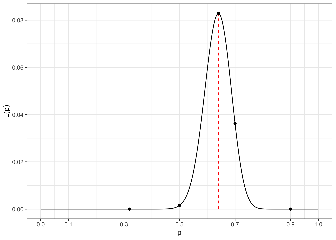

Figure 19.1: Likelihood function $L\left(p\right)$ when 64 heads are observed out of 100 coin flips.

19.1.2 Maximum Likelihood in Logistic Regression

We use this approach to calculate ${\hat{\beta }}_j$’s in logistic regression. The likelihood function for $n$ independent binary random variables can be written: $$L(p_1,\dots ,p_n)\propto \prod _{i=1}^n{p}_i^{y_i}(1-p_i{)}^{1-y_i}$$

Important differences from the coin flip example are that now $p_i$ is different for each observation and $p_i$ depends on $\beta$’s. Taking this into account, we can write the likelihood function for logistic regression as: $$L({\beta }_0,{\beta }_1,\dots ,{\beta }_k)=L\left(\beta \right)=\prod _{i=1}^n{p}_i\left(\beta {)}_i^y\right(1-p_i\left(\beta \right){)}^{1-y_i}$$ The goal of maximum likelihood is to find the values of $\beta$ that maximize $L\left(\beta \right)$. Our data have the highest probability of occurring when $\beta$ takes these values (compared to other values of $\beta$).

Unfortunately, there is not simple closed-form solution to finding $\hat{\beta }$. Instead, we use an iterative procedure called Iteratively Reweighted Least Squares (IRLS). This is done automatically by the glm() function in R, so we will skip over the details of the procedure.

If you want to know the value of the likelihood function for a logistic regression model, use the logLik() function on the fitted model object. This will return the logarithm of the likelihood. Alternatively, the summary output for glm() provides the deviance, which is $-2$ times the logarithm of the likelihood.

evans_glm <- glm(chd ~ age + ekg_abn + sbp + smoked,
                 data=evans, family=binomial)
logLik(evans_glm)

## 'log Lik.' -206.3872 (df=5)

19.2 Hypothesis Testing for $\beta$’s

Like with linear regression, a common inferential question in logistic regression is whether a ${\beta }_j$ is different from zero. This corresponds to there being a difference in the log odds of the outcome among observations that differen in the value of the predictor variable $x_j$.

There are three possible tests of $H_0:{\beta }_j=0$ vs. $H_A:{\beta }_j\ne 0$ in logistic regression:

• Likelihood Ratio Test
• Score Test
• Wald Test

In linear regression, all three are equivalent. In logistic regression (and other GLM’s), they are not equivalent.

19.2.1 Likelihood Ratio Test (LRT)

The LRT asks the question: Are the data significantly more likely when ${\beta }_j={\hat{\beta }}_j$ than when ${\beta }_j=0$? To do this, it compares the values of the log-likelihood for models with and without ${\beta }_j$ The test statistic is: $$\begin{array}{cc}\text{LR Statistic}\Lambda & =-2\log \frac{L\left(\widehat{reduced}\right)}{L\left(\widehat{full}\right)}\\ & =-2\log L\left(\widehat{reduced}\right)+2\log L\left(\widehat{full}\right)\end{array}$$

$\Lambda$ follows a ${\chi }_r^2$ distribution when $H_0$ is true and $n$ is large ($r$ is the number of variables set to zero, in this case $=1$). We reject the null hypothesis when $\Lambda >{\chi }_r^2\left(\alpha \right)$. This means that larger values of $\Lambda$ lead to rejecting $H_0$. Conceptually, if ${\beta }_j$ greatly improves the model fit, then $L\left(\widehat{full}\right)$ is much bigger than $L\left(\widehat{reduced}\right)$. This makes $\frac{L\left(\widehat{reduced}\right)}{L\left(\widehat{full}\right)}\approx 0$ and thus $\Lambda$ large.

A key advantage of the LRT is that the test doesn’t depend upon the model parameterization. We obtain same answer testing (1) $H_0:{\beta }_j=0$ vs. $H_A:{\beta }_j\ne 0$ as we would testing (2) $H_0:\exp \left({\beta }_j\right)=1$ vs. $H_A:\exp \left({\beta }_j\right)\ne 1$. A second advantage is that the LRT easily extends to testing multiple parmaeters at once.

Although the LRT requires fitting the model twice (once with all variables and once with the variables being tested held out), this is trivially fast for most modern computers.

19.2.2 LRT in R

To fit the LRT in R, use the anova(reduced, full, test="LRT") command. Here, reduced is the lm-object for the reduced model and full is the lm-object for the full model.

Example 19.3 Is there a relationship between smoking status and CHD among US men with the same age, EKG status, and systolic blood pressure (SBP)?

To answer this, we fit two models: one with age, EKG status, SBP, and smoking status as predictors, and another with only the first three.

evans_full <- glm(chd ~  age + ekg_abn + sbp + smoked,
                           data=evans,
                           family=binomial)
evans_red <- glm(chd ~  age + ekg_abn + sbp,
                           data=evans,
                           family=binomial)
anova(evans_red, evans_full, test="LRT")

## Analysis of Deviance Table
## 
## Model 1: chd ~ age + ekg_abn + sbp
## Model 2: chd ~ age + ekg_abn + sbp + smoked
##   Resid. Df Resid. Dev Df Deviance Pr(>Chi)   
## 1       605     421.23                        
## 2       604     412.77  1   8.4577 0.003635 **
## ---
## Signif. codes:  0 '***' 0.001 '**' 0.01 '*' 0.05 '.' 0.1 ' ' 1

We have strong evidence to reject that null hypothesis that smoking is not related to CHD in men, when adjusting for age, EKG status, and systolic blood pressure ($p=0.0036$).

19.2.3 Hypothesis Testing for $\beta$’s

19.2.4 Wald Test

A Wald test is, on the surface, the same type of test used in linear regression. The idea behind a Wald test is to calculate how many standard deviations ${\hat{\beta }}_j$ is from zero, and compare that value to a $Z$-statistic.

$$\begin{array}{cc}\text{Wald Statistic}W& =\frac{{\hat{\beta }}_j-0}{se\left({\hat{\beta }}_j\right)}\end{array}$$

$W$ follows a $N(0,1)$ distribution when $H_0$ is true and $n$ is large. We reject the $H:{\beta }_j=0$ when $|W|>z_{1-\alpha /2}$ or when $W^2>{\chi }_1^2\left(\alpha \right)$. That is, larger values of $W$ lead to rejecting $H_0$.

Generally, an LRT is preferred to a Wald test, since the Wald test has several drawbacks. A Wald test does depend upon the model parameterization: $$\frac{\hat{\beta }-0}{se\left(\hat{\beta }\right)}\ne \frac{\exp \left(\hat{\beta }\right)-1}{se\left(\exp \right(\hat{\beta }\left)\right)}$$ Wald tests can also have low power when truth is far from $H_0$ and are based on a normal approximation that is less reliable in small samples. The primary advantage to a Wald test is that it is easy to compute–and often provided by default in most statistical programs.

R can calculate the Wald test for you:

tidy(evans_full)

## # A tibble: 5 × 5
##   term        estimate std.error statistic  p.value
##   <chr>          <dbl>     <dbl>     <dbl>    <dbl>
## 1 (Intercept) -5.87      0.958       -6.13 8.98e-10
## 2 age          0.0415    0.0142       2.92 3.51e- 3
## 3 ekg_abn      0.465     0.289        1.61 1.07e- 1
## 4 sbp          0.00553   0.00462      1.20 2.31e- 1
## 5 smoked       0.837     0.302        2.77 5.62e- 3

19.2.5 Score Test

The score test relies on the fact that the slope of the log-likelihood function is 0 when $\beta =\hat{\beta }$¹⁷

The idea is to evaluate the slope of the log-likelihood for the “reduced” model (does not include ${\beta }_1$) and see if it is “significantly” steep. The score test is also called Rao test. The test statistic, $S$, follows a ${\chi }_r^2$ distribution when $H_0$ is true and $n$ is large ($r$ is the numnber of of variables set to zero, in this case $=1$). The null hypothesis is rejected when $S>{\chi }_r^2\left(\alpha \right)$.

An advantage of the score test is that is only requires fitting the reduced model. This provides computational advantages in some complex situations (generally not an issue for logistic regression). Like the LRT, the score test doesn’t depend upon the model parameterization

Calculate the score test using with test="Rao"

anova(evans_red, evans_full, test="Rao")

## Analysis of Deviance Table
## 
## Model 1: chd ~ age + ekg_abn + sbp
## Model 2: chd ~ age + ekg_abn + sbp + smoked
##   Resid. Df Resid. Dev Df Deviance    Rao Pr(>Chi)   
## 1       605     421.23                               
## 2       604     412.77  1   8.4577 7.9551 0.004795 **
## ---
## Signif. codes:  0 '***' 0.001 '**' 0.01 '*' 0.05 '.' 0.1 ' ' 1

19.3 Interval Estimation

There are two ways for computing confidence intervals in logistic regression. Both are based on inverting testing approaches.

19.3.1 Wald Confidence Intervals

Consider the Wald hypothesis test:

$$W=\frac{{\hat{\beta }}_j-{\beta }_j^0}{se\left({\hat{\beta }}_j\right)}$$ If $|W|\ge z_{1-\alpha /2}$, then we would reject the null hypothesis $H_0:{\beta }_j={\beta }_j^0$ at the $\alpha$ level.

Reverse the formula for $W$ to get:

$${\hat{\beta }}_k-z_{1-\alpha /2}se\left({\hat{\beta }}_j\right)\le {\beta }_j^0\le {\hat{\beta }}_k+z_{1-\alpha /2}se\left({\hat{\beta }}_j\right)$$

Thus, a $100\times (1-\alpha )\%$ Wald confidence interval for ${\beta }_j$ is:

$$({\hat{\beta }}_k-z_{1-\alpha /2}se({\hat{\beta }}_j),{\hat{\beta }}_k+z_{1-\alpha /2}se({\hat{\beta }}_j\left)\right)$$

19.3.2 Profile Confidence Intervals

Wald confidence intervals have a simple formula, but don’t always work well–especially in small sample sizes (which is also when Wald Tests are not as good). Profile Confidence Intervals “reverse” a LRT similar to how a Wald CI “reverses” a Wald Hypothesis test.

• Profile confidence intervals are usually better to use than Wald CI’s.
• Interpretation is the same for both.
• In R, the command confint() uses profile CI’s for logistic regression.
  • This is also what tidy() will use when conf.int=TRUE

To get a confidence interval for an OR, exponentiate the confidence interval for ${\hat{\beta }}_j$

exp(confint(evans_full, level = 0.95))

## Waiting for profiling to be done...

##                    2.5 %   97.5 %
## (Intercept) 0.0004138279 0.017891
## age         1.0136806045 1.071868
## ekg_abn     0.8946658909 2.785309
## sbp         0.9963253392 1.014616
## smoked      1.3034626923 4.290179

19.4 Generalized Linear Models (GLMs)

Logistic regression is one example of a generalized linear model (GLM). GLMs have three pieces:

GLM Part	Explanation	Logistic Regression
Probability Distribution from Exponential Family	Describes generating mechanism for observed data and mean-variance relationship.	$Y_i\sim Bernoilli\left(p_i\right)$ $Var\left(Y_i\right)\propto p_i(1-p_i)$
Linear Predictor $\eta =X\beta$	Describes how $\eta$ depends on linear combination of parameters and predictor variables	$\eta =X\beta$
Link function $g$. $E\left[Y\right]=g^{-1}\left(\eta \right)$	Connection between mean of distribution and linear predictor	$p=\frac{\exp \left(\eta \right)}{1+\exp \left(\eta \right)}$ or $logit\left(p\right)=\eta$

Another common GLM is Poisson regression (“log-linear” models)

GLM Part	Explanation	Poisson Regression
Probability Distribution from Exponential Family	Describes generating mechanism for observed data and mean-variance relationship.	$Y_i\sim Poisson\left({\lambda }_i\right)$ $Var\left(Y_i\right)\propto {\lambda }_i$
Linear Predictor $\eta =X\beta$	Describes how $\eta$ depends on linear combination of parameters and predictor variables	$\eta =X\beta$
Link function $g$. $E\left[Y\right]=g^{-1}\left(\eta \right)$	Connection between mean of distribution and linear predictor	${\lambda }_i=\exp \left(\eta \right)$ or $\log \left({\lambda }_i\right)=\eta$

---

16. The value of the constant is a binomial coefficient, but it’s exact value is not important for our needs here.↩︎

17. This follows from the first derivative of a function always equally zero at a local extremum.↩︎