Chapter 6 Inference for the SLR Model
\(\newcommand{\E}{\mathrm{E}}\) \(\newcommand{\Var}{\mathrm{Var}}\)
In Chapter 4 we saw how to conduct inference about the parameters \(\beta_0\) and \(\beta_1\). That allowed to answer quesitons about the nature of the relationship between \(x_i\) and \(y_i\).
A related question we might ask is: Is the model useful overall? Rather than testing a specific parameter, this questions asks about the overall utility of the entire regression model. In this chapter, we explore how to address this question using F-tests.
6.1 Sum of Squares Decomposition
Decomposing the variability in the data provides the pieces necessary to assess overall model performance. The total variability in outcome for a specific dataset is given by the sample variance of the \(y_i\)’s. In regression this quantity is commonly called the total sum of squares:
\[SS_{tot} = \displaystyle\sum_{i=1}^n(y_i - \overline{y})^2\]
This is the sum of the squared distances between each observation and the overall mean, which can be visually represented by the sum of the squared lengths of the green lines in Figure 6.1.
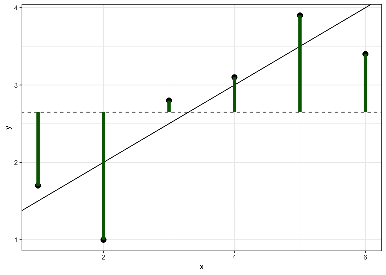
Figure 6.1: Simulated data showing \(SS_{tot}\), which is the sum of the squared lengths of the green lines.
The total sum of squares can be decomposed into two pieces:
\[\begin{align} \sum_{i=1}^n (y_i - \overline{y})^2 &= \sum_{i=1}^n \left(y_i - \hat y_i + \hat y_i - \overline{y}\right)^2 \notag\\ &= \sum_{i=1}^n (y_i - \hat y_i)^2 + 2 \sum_{i=1}^n(y_i - \hat y_i)(\hat y_i - \overline{y}) + \sum_{i=1}^n (\hat y_i - \overline y)^2 \notag\\ &= \sum_{i=1}^n (y_i - \hat y_i)^2 + 2 \sum_{i=1}^n(y_i - \hat y_i)\hat y_i \notag \\ & \qquad \qquad \qquad - 2 \sum_{i=1}^n(y_i - \hat y_i)\overline{y}+ \sum_{i=1}^n (\hat y_i - \overline y)^2 \notag\\ &= \sum_{i=1}^n (y_i - \hat y_i)^2 + \sum_{i=1}^n (\hat y_i - \overline y)^2 \tag{6.1} \end{align}\] The first term in (6.1) is called the residual sum of squares:
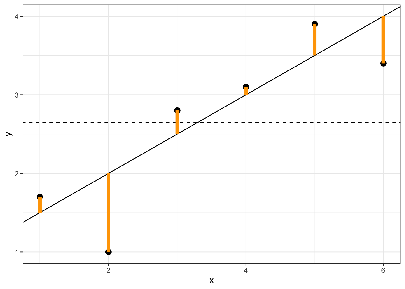
\[SS_{res} = \sum_{i=1}^n (y_i - \hat y_i)^2\]
This should look familiar–it is the same things as the sum of squared residuals (\(\sum_{i=1}^n e_i^2 = (n-2)\hat\sigma^2\)). This is variability “left over” from fitted regression model, and can be visualized as the sum of the squared distances in the following figure:
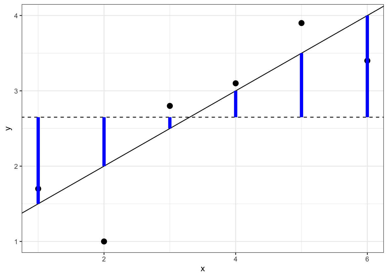
The other term in (6.1) is the regression sum of squares: \[SS_{reg} = \sum_{i=1}^n (\hat y_i - \overline y)^2\]. This is the variability that is explained by the regression model:
6.2 Coefficient of Determination (\(R^2\))
One way to determine how “good” a model fit is, is to compute the proportion of variability in the outcome that is accounted for by the regression model. This can be represented by the following ratio:
\[\frac{SS_{reg}}{SS_{tot}} = 1 - \frac{SS_{res}}{SS_{tot}} = R^2\] The quantity \(R^2\) is commonly called the coefficient of determination. The denominator \(SS_{tot}\) is a fixed quantity and the numerator \(SS_{reg}\) can vary by model (i.e., by the chosen predictor variable). Larger values of \(R^2\) mean that greater amounts of variability in the outcome is explained by the model. When there are multiple predictor variables in a model, we will need to use an alternative form of \(R^2\) (see Section 10.7).
Since the amount of variation explained by the model cannot be greater than the total variation in the outcome, \(R^2\) must lie between 0 and 1. The range of \(R^2\) values corresponding to a “good” or “bad” model fit varies by context. In most settings, values above 0.8 represent a “good” model. But in some contexts, \(R^2\) as low as 0.3 can be “good”. What is “good” for prediction may differ from what is “good” for learning about the underlying science, and vice versa. Making a qualitative judgment about \(R^2\) requires familiarity with what is typical for the type of data being analyzed.
R will compute the value of \(R^2\) for you in the output from summary():
##
## Call:
## lm(formula = body_mass_g ~ flipper_length_mm, data = penguins)
##
## Residuals:
##      Min       1Q   Median       3Q      Max
## -1058.80  -259.27   -26.88   247.33  1288.69
##
## Coefficients:
##                    Estimate Std. Error t value Pr(>|t|)
## (Intercept)       -5780.831    305.815  -18.90   <2e-16 ***
## flipper_length_mm    49.686      1.518   32.72   <2e-16 ***
## ---
## Signif. codes:  0 '***' 0.001 '**' 0.01 '*' 0.05 '.' 0.1 ' ' 1
##
## Residual standard error: 394.3 on 340 degrees of freedom
##   (2 observations deleted due to missingness)
## Multiple R-squared:  0.759,  Adjusted R-squared:  0.7583
## F-statistic:  1071 on 1 and 340 DF,  p-value: < 2.2e-16
The value of \(R^2\) is listed as Multiple R-squared: 0.759 in the second line from the bottom. Adjusted \(R^2\) will be discussed in Section 10.7.
6.3 F-Test for Regression
In regression, we can ask whether there is an overall linear relationship between the predictor variable and the average values of the outcome variable. This is commonly called a test for significance of regression or a global F-test, and the corresponding null and alternative hypotheses are:
- \(H_0 =\) There is no linear relationship between the \(x\)’s and the average value of \(y\)
- \(H_A =\) There is a linear relationship between the \(x\)’s and the average value of \(y\)
In SLR there is only one \(x\) variable, so this is exactly equivalent to testing \(H_0: \beta_1 = 0\) vs. \(H_A: \beta_1 \ne 0\). However, when there are multiple predictor variables in the model, the global F-test and a test for a single \(\beta\) parameter are no longer the same (see Section 10.5).
The test statistic for the test for significance of regression is:
\[\begin{equation} \label{eq:slrfstat} f = \frac{MS_{reg}}{MS_{res}} = \frac{SS_{reg}/df_{reg}}{SS_{res}/df_{res}} = \frac{SS_{reg}/1}{SS_{res}/(n-2)} \end{equation}\]
In equation (??), the statistic can be heuristically thought of as a signal-to-noise ratio. The numerator \(SS_{reg}/1\) is the average amount of variabiliy explained by each predictor variable, which is a measure of “signal”. The denominator \(SS_{res}/(n-2)\) is the average amount of variability left unexplained, which is a measure of “noise”.
When the value of \(f\) is large enough, we conclude that the variability explained by the model is sufficiently larger than the variability left unexplained. Thus, we use a one-sided test and reject \(H_0\) if \(f\) is large enough. If the null hypothesis is true and the \(\epsilon_i\) are normally distributed,8 then \(f\) follows an \(F\) distribution with 1 and \(n-2\) degrees of freedom, i.e., \(f \sim F_{1, n-2}\).
6.3.1 F-test in R “by hand”
Example 6.1 In the penguin data from Example 4.7, is there a linear relationship between flipper length and body mass?
To answer this using a global F-test, we set up the null and alternative hypotheses as:
\(H_0 =\) There is no linear relationship between penguin flipper length and average body mass.
\(H_A =\) There is a linear relationship between penguin flipper length and average body mass.
We now need to compute \(SS_{res}\):
## [1] 52854796and \(SS_{reg}\):
## [1] 166452902Note that when computing \(SS_{reg}\) in this way, we are using penguin_lm$model$body_mass_g rather than penguins$body_mass_g. This is because the version of body mass stored within the penguin_lm object will contain exactly the observations used to fit the model. This can be important if there is missing data that lm() drops automatically.
With both \(SS_{res}\) and \(SS_{reg}\) calculated, we can compute the F-statistic:
## [1] 1070.745and \(p\)-value (being careful to set lower=FALSE to do a one-sided test):
## [1] 4.370681e-1076.3.2 F-test in R
Of course, it is faster and simpler to let R compute the F-statistic and \(p\)-value for you. This information is available at the bottom of the output from summary():
##
## Call:
## lm(formula = body_mass_g ~ flipper_length_mm, data = penguins)
##
## Residuals:
##      Min       1Q   Median       3Q      Max
## -1058.80  -259.27   -26.88   247.33  1288.69
##
## Coefficients:
##                    Estimate Std. Error t value Pr(>|t|)
## (Intercept)       -5780.831    305.815  -18.90   <2e-16 ***
## flipper_length_mm    49.686      1.518   32.72   <2e-16 ***
## ---
## Signif. codes:  0 '***' 0.001 '**' 0.01 '*' 0.05 '.' 0.1 ' ' 1
##
## Residual standard error: 394.3 on 340 degrees of freedom
##   (2 observations deleted due to missingness)
## Multiple R-squared:  0.759,  Adjusted R-squared:  0.7583
## F-statistic:  1071 on 1 and 340 DF,  p-value: < 2.2e-16
Regardless of which approach to calculating the test statistic that we use, we can summarize our conclusions by saying:
We reject the null hypothesis that there is no linear relationship between penguin flipper length and average body mass (\(p < 0.0001\)).
6.4 ANOVA Table
\(F\)-tests are widely used in the Analysis of Variance (ANOVA) approach to analyzing data. Information can be summarized in an “ANOVA Table”:
| Source of Variation | Sum of Squares | Degrees of Freedom | MS | F |
|---|---|---|---|---|
| Regression | \(SS_{reg}\) | \(1\) | \(MS_{reg}\) | \(MS_{reg}/MS_{res}\) |
| Residual | \(SS_{res}\) | \(n-2\) | \(MS_{res}\) | – |
| Total | \(SS_{tot}\) | \(n-1\) | – | – |
This format arises most frequently for designed experiments, where there is a rich history of decomposing the variability of data into distinct sources.
In many cases, it is sufficient for sample sizes to be large so that the central limit theorem applies. But care should be taken in small samples.↩︎