Chapter 12 Assessing Model Assumptions
\(\newcommand{\E}{\mathrm{E}}\) \(\newcommand{\Var}{\mathrm{Var}}\) \(\newcommand{\bme}{\mathbf{e}}\) \(\newcommand{\bmx}{\mathbf{x}}\) \(\newcommand{\bmH}{\mathbf{H}}\) \(\newcommand{\bmI}{\mathbf{I}}\) \(\newcommand{\bmX}{\mathbf{X}}\) \(\newcommand{\bmy}{\mathbf{y}}\) \(\newcommand{\bmY}{\mathbf{Y}}\) \(\newcommand{\bmbeta}{\boldsymbol{\beta}}\) \(\newcommand{\bmepsilon}{\boldsymbol{\epsilon}}\) \(\newcommand{\bmmu}{\boldsymbol{\mu}}\) \(\newcommand{\bmSigma}{\boldsymbol{\Sigma}}\) \(\newcommand{\XtX}{\bmX^\mT\bmX}\) \(\newcommand{\mT}{\mathsf{T}}\) \(\newcommand{\XtXinv}{(\bmX^\mT\bmX)^{-1}}\)
12.1 Residuals
The residuals for a model are the difference between the predicted value and the true observation. Each residual gives an estimate of the error \(\epsilon_i\). Since the residuals provide information about how close the model is to the observed values, they can be used to assess violations of the model assumptions, as we will see below.
There are four types of residuals: raw, scaled, standardized, and studentized.
12.1.1 Raw Residuals
Raw residuals are the difference between the observed values (\(y_i\)) and the fitted values (\(\hat y_i)\): \[e_i = y_i - \hat y_i\]
In general, the term “residuals”–without more specification–refers to these values. For simple linear regression, these values can be seen directly on a scatterplot, by calculating the vertical distance between each point and the regression line. In multiple linear regression, they conceptual idea is the same, but it is not as easy to visualize them.
In R, these can be obtained using the function residuals().
Example 12.1 Consider a simple linear regression model fit to the fuel efficiency data introduced in Section 1.3.5, with highway fuel efficiency as the outcome and engine displacement as the predictor variable. Figure 12.1 shows the observations and the regression line; the residuals are the distances along the red lines connecting each point to the regression line.
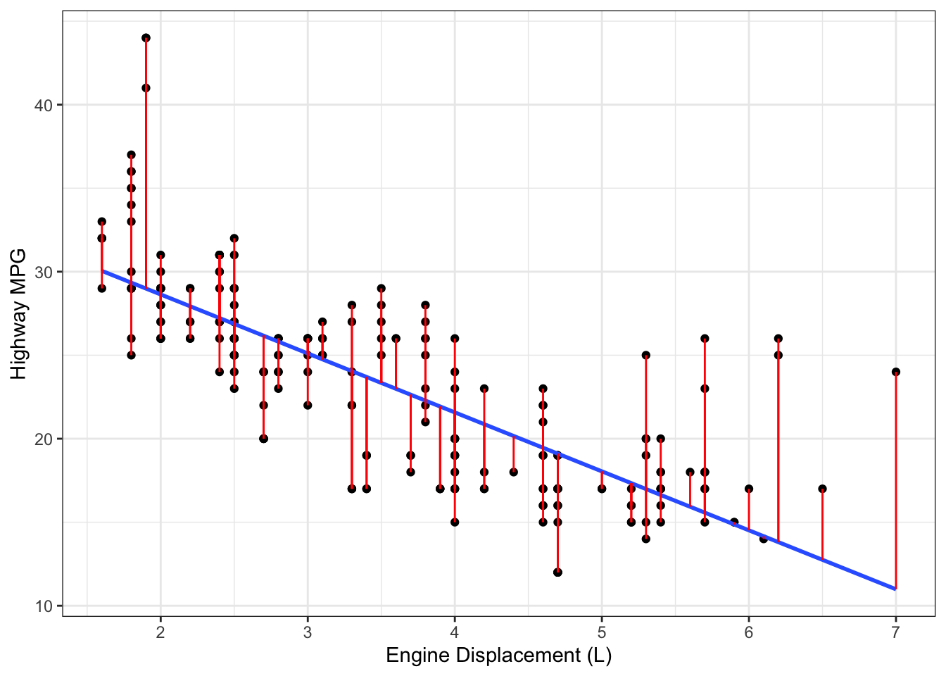
Figure 12.1: Data, regression line (black) and residuals (red) from a simple linear regression fit to fuel efficiency data.
12.1.2 Scaled Residuals
The magnitude of the raw residuals depends on \(\sigma^2\), which can make them difficult to compare across models. Dividing by the estimated residual variance (\(\sqrt{\hat\sigma^2}\)) puts residuals on a comparable scale and yields scaled residuals:
\[d_i = \frac{e_i}{\sqrt{\hat\sigma^2}}\]
12.1.3 Standardized Residuals
But we can do better scaling than this. The residual standard error \(\hat\sigma^2\) is a global estimate of \(\sigma^2\), but not the best estimate of the variance of the \(i\)th residual (\(\Var(e_j)\)).
To find \(\Var(e_i)\), we first find \(\Var(\bme)\): \[\begin{align*} \Var(\mathbf{e}) &= \Var((\bmI - \bmH)\bmy)\\ &= (\bmI - \bmH) \Var(\bmy)(\bmI - \bmH)^\mT\\ &= (\bmI - \bmH) \sigma^2(\bmI - \bmH)^\mT\\ &= \sigma^2 (\bmI - \bmH)(\bmI - \bmH)\quad \{(\bmI - \bmH) = (\bmI - \bmH)^\mT\}\\ &= \sigma^2 (\bmI\bmI - \bmH\bmI - \bmI\bmH + \bmH\bmH)\\ &= \sigma^2 (\bmI - \bmH) \quad \text{\{since $\bmH$ is idempotent\}} \end{align*}\] It immediately follows that \(\Var(e_i) = \sigma^2 (1-h_{ii})\).
The value of \(h_{ii}\), the \(i\)th diagonal element of the hat matrix (Section 9.8), is larger for points that are more remote in predictor space. Remote points have smaller residual variance, since they “pull” the regression line more towards themselves. This idea, which we will revisit in the discussion of leverage in Section 13, is illustrated in Figure 12.2. Since
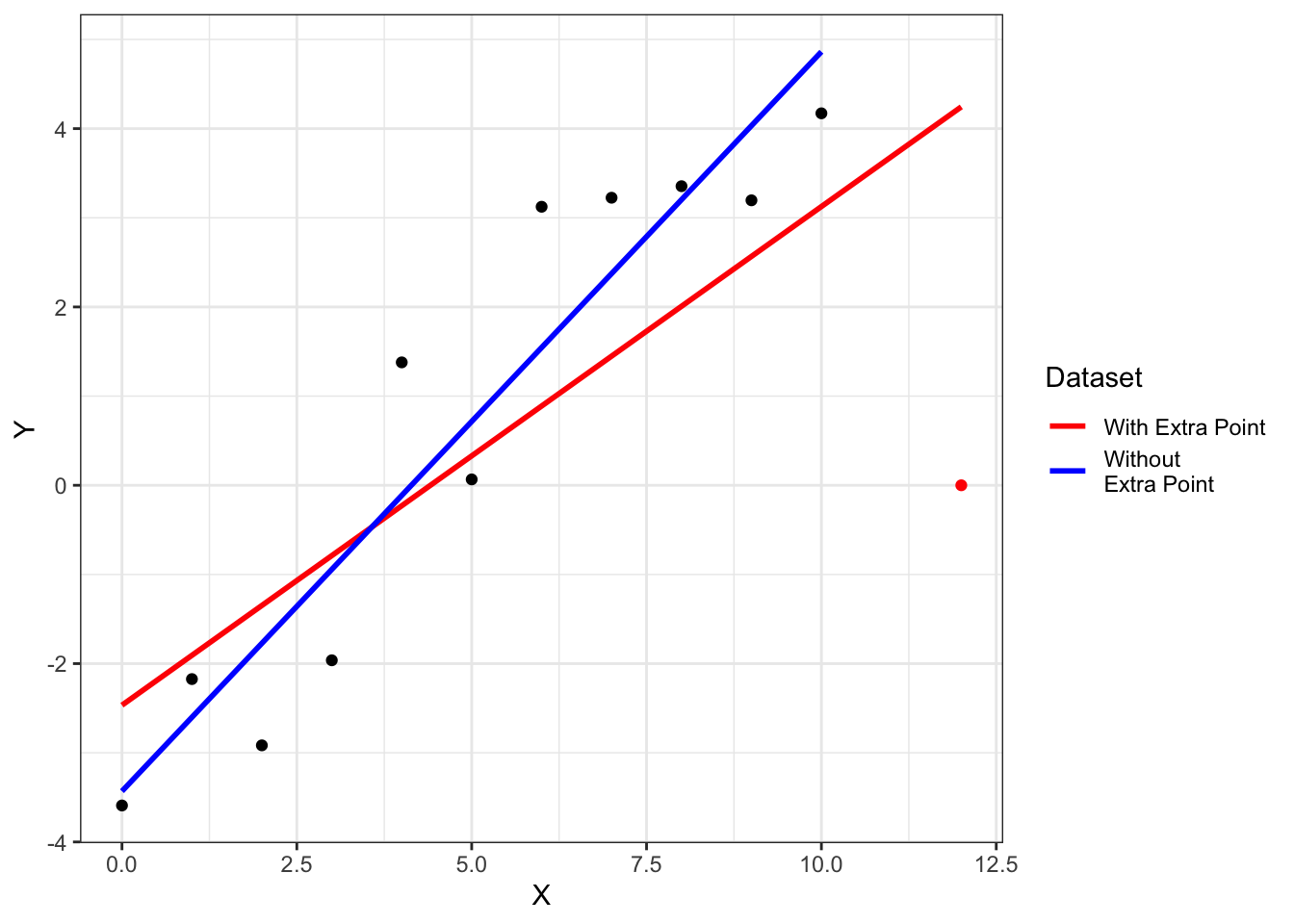
Figure 12.2: Regression line fit to data with and without the extra point at \(x=12\).
Dividing \(e_i\) by its estimated variance yields the standardized residuals:
\[r_i = \frac{e_i}{\sqrt{\hat\sigma^2(1 - h_{ii})}}\]
One advantage of standardized residuals is that they have variance equal to 1. This makes them simple to compare across model fits.
12.1.4 Studentized Residuals
The last type of residual, the studentized residual, provides a better way for detecting an outlier. Standardized residuals include the current observation when computing \(\hat\sigma^2\) (which is used in the estimated value of \(\Var(e_i)\)). To better detect outliers, we can compute \(\hat\sigma_{(i)}^2\), which is the estimated residual variance when leaving out observation \(i\).
This gives the studentized residuals:
\[t_i = \frac{e_i}{\sqrt{\hat\sigma^2_{(i)}(1 - h_{ii})}}\]
Studentized residuals follow a \(T_{n - p - 1}\) distribution.
12.1.5 Residuals Summary
The different types of residuals are summarizedd in the following table:
| Type of Residual | Value | R Command |
|---|---|---|
| (Raw) residual | \(e_i = y_i - \hat y_i\) | residuals() |
| Scaled residual | \(d_i = \dfrac{e_i}{\sqrt{\hat\sigma^2}}\) | (none) |
| Standardized residual | \(r_i = \dfrac{e_i}{\sqrt{\hat\sigma^2(1 - h_{ii})}}\) | rstandard() |
| Studentized residual | \(t_i = \dfrac{e_i}{\sqrt{\hat\sigma^2_{(i)}(1 - h_{ii})}}\) | rstudent() |
12.2 MLR Model Assumptions
In Section 9.2, we introduced the matrix form for the multiple linear regression model: \[\begin{align} \mathbf{y} &= \mathbf{X}\boldsymbol{\beta} + \boldsymbol{\epsilon}\\ \E[\bmepsilon] &= \mathbf{0} \\ \Var[\bmepsilon] &= \sigma^2\bmI \\ \bmX & \text{ is `full-rank'} \end{align}\]
So far, we have focused on how to interpret, estimate, and test the model parameters and paid little attention to the model assumptions. Now we will take a closer look at each of these assumptions and how to evaluate if they hold in our data.
12.2.1 Assumption 1: \(\E[\bmepsilon] = \mathbf{0}\)
This assumption has two consequences. The first is that the errors \(\epsilon_i\) have mean zero. This is ensured by the inclusion of the intercept in the model. The second consequence is that the relationship between the mean of the repsonse and the predictors is (approximately) linear. That is, that \(\E[\bmy] = \bmX\bmbeta\). Violations of this assumption can lead to results that are misleading and incorrect, since the trend being modeled does not match the trend in the data.
We can assess this assumption by plotting standardized residuals (\(s_i\)) against fitted values (\(\hat y_i\)). While a violation of the linearity assumption can take different forms, the most common is a curved or “bow” pattern. The bow pattern (right side of Figure 12.3) arises when there is a quadratic or exponential-type shape (left side of Figure 12.3).
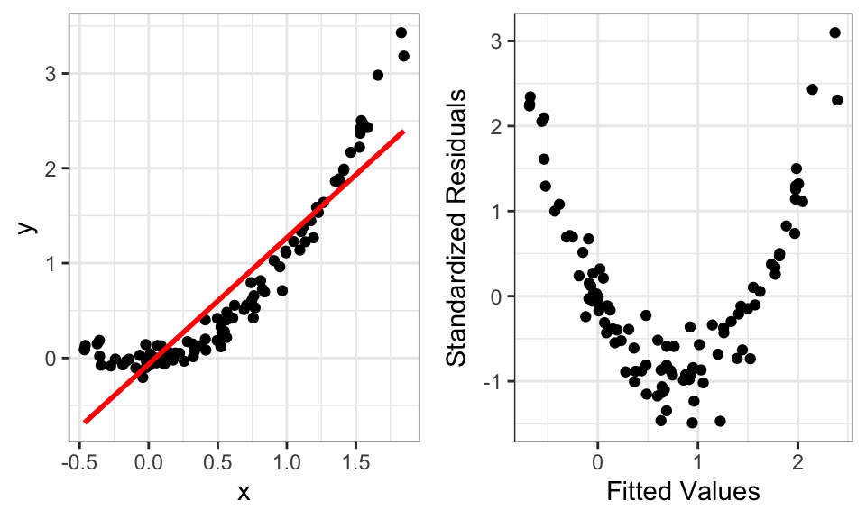
Figure 12.3: Data (left) and residual-fitted plot (right) that violates the linearity assumption.
12.2.2 Assumption 2: \(\Var(\epsilon_i) = \sigma^2 \text{ for } i=1, \dots, n\)
This assumption means that the errors \(\epsilon_i\) have constant variance. Violations of this assumption don’t impact the regression line itself, but can have major effects on the estimated variance \(\hat\sigma^2\). This can lead to improper inference and incorrect confidence intervals.
A plot of standardized residuals (\(s_i\)) against fitted values (\(\hat y_i\)) can be used to address this assumption as well. Violations of this assumption are most often evident as a “cone” pattern in the residuals, wherein the spread of residuals differs by fitted value (Figure 12.4).
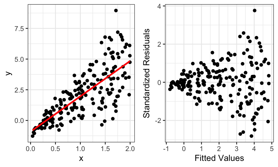
Figure 12.4: Data (left) and residual-fitted plot (right) that violates the constant variance assumption.
12.2.3 Assumption 3: \(Cov(\epsilon_i, \epsilon_j) = 0 \text{ for } i\ne j\)
This assumption, which is a consequence of \(\Var(\bmepsilon) = \sigma^2\bmI\), means that the observations are uncorrelated. If the observations are correlated, then the estimated variances will be incorrect. This can lead to improper inference and incorrect confidence intervals.
Unfortunately, this assumption can not be easily assessed using residual plots. In some special cases, such as with time series or spatial data, this can be diagnosed. But in many cases, this assumption relies on understanding how the data were collected.
12.2.4 Assumption 4: \(\bmX\) is full-rank.
As discussed in Section 9.4, this is a mathematical requirement for estimating \(\hat\beta\).13 Practically, R will drop collinear columns so that this is not an issue. But it is good practice to not intentionally set up a model that has linear dependent predictor variables. This is perhaps most common in models with extensive interactions and indicator variables, since they lead to many derived variables.
12.2.5 Assumption 5: \(\epsilon_i\) are approximately normally distributed.
This assumption is necessary for the correct distributions of the test statistics under the null hypothesis. In Section 4.3, we explained how the Central Limit Theorem assures us of approximate normalty in large samples, although it’s always a good idea to check this assumption. If violated, the results from hypothesis tests and confidence intervals can be incorrect, although the regression coefficients \(\hat\bmbeta\) are still valid.
To assess the normality of residuals, we can use a QQ plot, which plots the quantiles of the sample distribution against quantiles of the standard normal distribution. If the sample is from an approximately normal distribution, then the points will line up on the 1-1 line (Figure 12.5). Deviation from the 1-1 line indicates lack of normality (Figure 12.6).
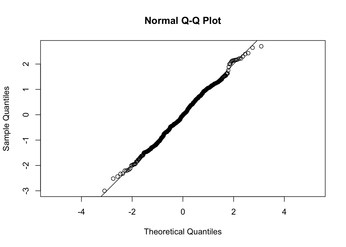
Figure 12.5: QQ plot for a sample from the Normal distribution.
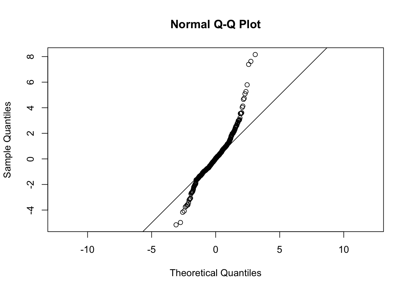
Figure 12.6: QQ plot for a sample a distribution that is not normal.
12.2.6 Examples
Example 12.2 We have data on stock prices from the S&P 500 on February 8, 2018, including the stock price and market capitalization. Consider an SLR model with market capitalization as the predictor variable and stock price as the outcome. Is there evidence of violation of any of the model assumptions?
To answer this, let’s first plot the data with the regression line. Figure 12.7 shows the data, and it is clearly evident that the values of both variables are skewed. (In Section 14, we’ll revisit this data to see how a transformation can fix this).
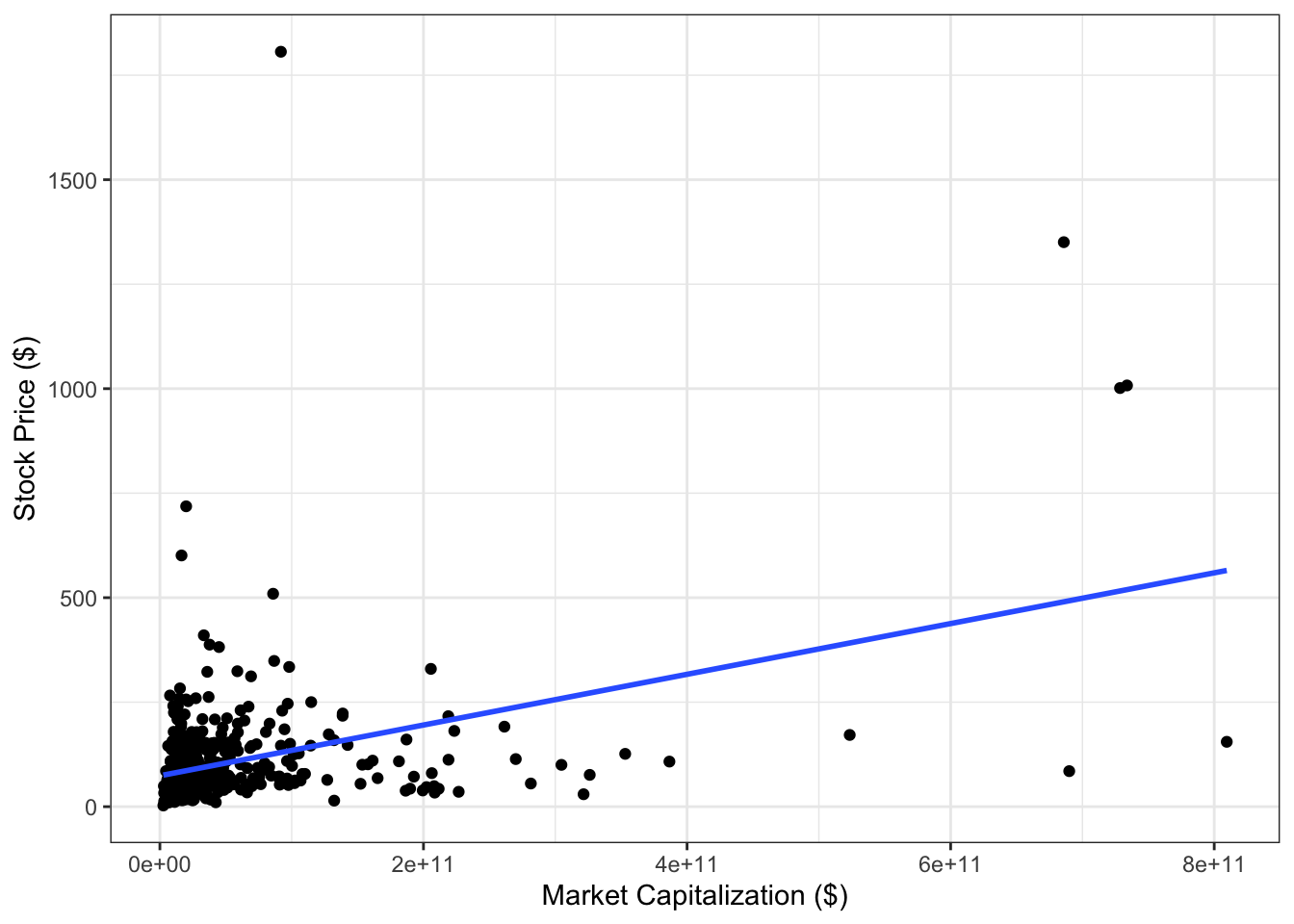
Figure 12.7: Scatter plot of stock prices and market capitalization.
The residual-fitted plot is shown in Figure 12.8. There is a clear downward trend in the residuals, which is evidence of violation of the linearity assumption. It is difficult to determine if there is violation of the constant variance assumption, given the small number of data points with large fitted values.
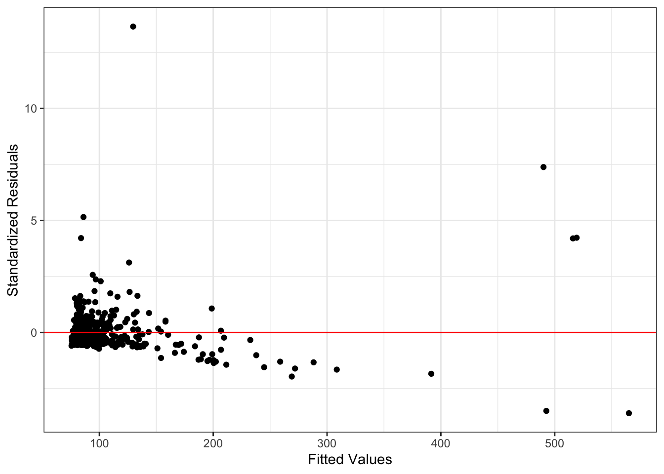
Figure 12.8: Residuals versus fitted values in regression model for stock price data.
Figure12.9 shows evidence of non-normality in the residuals. Since we are already planning on using model transformations to fix the other violated assumptions, we can wait to re-evaluate this one again in those models.
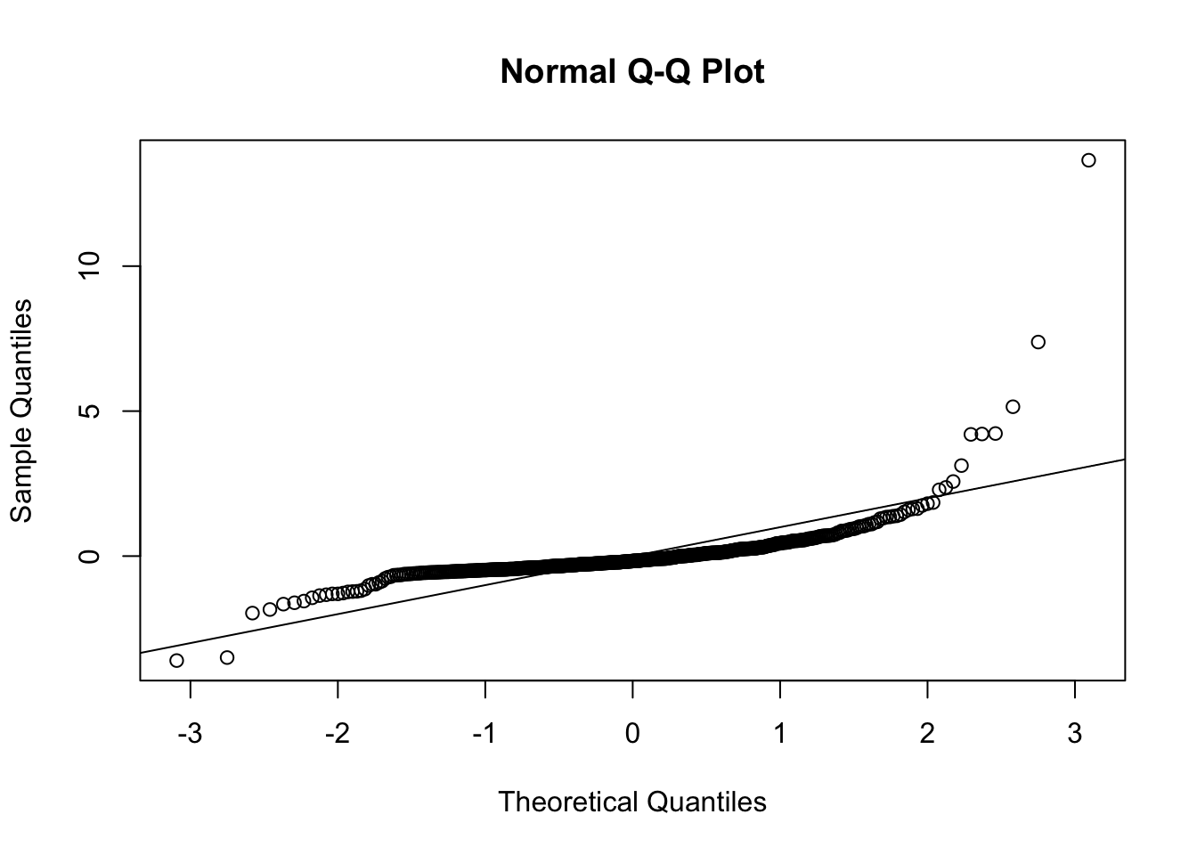
Figure 12.9: QQ plot for residuals in regression model for stock price data.
In fact, there are methods to get around this constraint, but those are beyond the scope of this text.↩︎