Chapter 5 Inference and Prediction for the Mean Response in SLR
\(\newcommand{\E}{\mathrm{E}}\) \(\newcommand{\Var}{\mathrm{Var}}\) \(\newcommand{\bmx}{\mathbf{x}}\) \(\newcommand{\bmX}{\mathbf{X}}\)
5.1 Estimating Mean & Predicting Observations
5.1.1 Estimation or Prediction?
In Section 2.3.5 we saw that the values along the regression line can be interpeted as the mean outcome for a given value of the predictor variable. Formally, we can write the estimated mean of \(Y\) when \(x\) equals some value \(x_0\) as:
\[\begin{equation} \hat\mu_{Y|x_0} = \hat\beta_0 + \hat\beta_1x_0 \tag{5.1} \end{equation}\]
The points along the line also provide the best prediction of the value of \(Y\) for an observation with \(x=x_0\). We write the prediction for a new observation of \(Y\) when \(x\) equals some value \(x_0\) as:
\[\begin{equation} \hat y_0 = \hat\beta_0 + \hat\beta_1x_0 \tag{5.2} \end{equation}\]
Although very similar, there an important distinction between the questions
- What is the mean value of \(Y\) when \(x=x_0\)?
- What is the value of a new observation with \(x=x_0\)?
The point estimate for these questions is the same, but the corresponding uncertainty is different. Question 1 is answered by \(\hat\mu_{Y|x_0}\) and has a corresponding confidence interval. Question 2 is answered by \(\hat y_0\) and has a corresponding prediction interval.
5.1.2 Computing \(\hat\mu_{Y|x_0}\) and \(\hat{y}_0\)
The point estimates \(\hat\mu_{Y|x_0}\) and \(\hat{y}_0\) can be computed by directly plugging in the point estimates to (5.1) or (5.2).
Example 5.1 In Example 3.1, we saw the fitted regression line for mean penguin body mass (\(y\)) as a function of flipper length (\(x\)) was: \[\hat{y} = -5780.83 + 49.69x\] Using this model, what is the mean body mass for a penguin with flipper length of 200mm?
Solution. (Version 1) We can compute these directly from the model objects:
## (Intercept)
## 4156.282From this, we obtain the estimated mean as 4,156 grams.
But rather than compute this value using addition and multiplication, we can use the predict() function in R, which will compute these values for us based on a fitted lm object. The necessary arguments for making predictions are:
object=, thelmfor the model you want to make predictions fornewdata=, a data frame containing the named variables with the values for prediction
Solution. (Version 2 for Example 5.1.) Rather than do the arithmetic by hand, we can use the predict() function. We create a data frame called preddata that contains the information for prediction, and then pass it to predict().
penguin_lm <- lm(body_mass_g ~ flipper_length_mm,
   data=penguins)
preddata <- data.frame(flipper_length_mm=200)
predict(penguin_lm,
newdata=preddata)## 1
## 4156.282We again obtain the estimated mean as 4,156 grams.
In addition to being less likely to lead to typos, using the predict() command is easily scalable to multiple values.
Example 5.2 For the same model as Example 5.1, what is the predicted mean body mass for penguins with flipper lengths of 150mm, 200mm, 225mm, and 250mm?
Solution. We can create a data frame with muliple values and then make predictions using that data frame:
preddata2 <- data.frame(flipper_length_mm=c(150, 200, 225, 250))
predict(penguin_lm,
        newdata=preddata2)
## 1 2 3 4
## 1672.004 4156.282 5398.421 6640.5605.2 Inference for the mean (\(\mu_{Y|x_0}\))
5.2.1 CIs and Testing
Confidence intervals for \(\mu_{Y | x_0}\) can be constructed in the same way as for the \(\beta\)’s:
\[\begin{equation} \left(\hat\mu_{y|x_0} - t_{\alpha/2}\widehat{se}(\hat\mu_{y|x_0}), \hat\mu_{y|x_0} + t_{\alpha/2}\widehat{se}(\hat\mu_{y|x_0})\right). \tag{5.3} \end{equation}\]
Hypothesis testing for the mean response is much less common, since inference is usually done on the regression slope (\(\beta_1\)) or the model overall (Section 6). But if needed, it is also conducted in a manner analogous to the \(\beta\)’s:
\[H_0: \mu_{y|x_0} = \mu^0_{y|x_0} \qquad \text{vs.} \qquad H_A: \mu_{y|x_0} \ne \mu^0_{y|x_0}\]
\[\begin{equation} t = \frac{\hat\mu_{y|x_0} - \mu^0_{y|x_0}}{\widehat{se}(\hat\mu_{y|x_0})} \tag{5.4} \end{equation}\]
5.2.2 Variance of \(\hat\mu_{y|x_0}\)
Computing either the confidence interval (5.3) or the test statistic (5.4) requires computing the standard erorr \(\widehat{se}(\hat\mu_{y|x_0})\).
We can compute the variance of \(\hat\mu_{y|x_0}\) as follows:
\[\begin{align} \Var(\hat\mu_{y|x_0}) &= \Var\left(\hat\beta_0 + \hat\beta_1 x_0 \right)\\ & = \Var\left(\overline{y} - \hat\beta_1\overline{x} + \hat\beta_1 x_0 \right) \tag{5.5}\\ & = \Var\left(\overline{y} + \hat\beta_1(x_0 - \overline{x} )\right)\\ & = \Var\left(\overline{y}\right) + \Var\left(\hat\beta_1(x_0 - \overline{x}) \right)\notag\\ & = \frac{\sigma^2}{n} + (x_0 - \overline{x})^2\Var\left(\hat\beta_1\right)\notag\\ & = \frac{\sigma^2}{n} + (x_0 - \overline{x})^2\frac{\sigma^2}{S_{xx}}\notag\\ & = \sigma^2\left(\frac{1}{n} + \frac{(x_0 - \overline{x})^2}{S_{xx}}\right) \tag{5.6} \end{align}\]
It is important to note that \(\Var\left(\hat\beta_0 + \hat\beta_1 x_0 \right) \ne \Var(\hat\beta_0) + \Var(\hat\beta_1x_0)\) since the estimators \(\hat\beta_0\) and \(\hat\beta_1\) are correlated. To obtain (5.5), we have substituted in \(\hat\beta_0 = \overline{y} - \hat\beta_1\overline{x}\) (recall equation (3.4)).
The variance (5.6) changes as a function of \(x\) and is minimized when \(x_0 = \overline{x}\). This corresponds with what our intuition might tell us: that there is the least uncertainty near the center of the data.
5.2.3 Computing the CI for Mean Response
5.2.3.1 “By Hand”
Using equation (5.6), we can directly compute \(\widehat{se}(\hat\mu_{y|x_0})\) and derive a confidence interval.
# Be careful with missing values here
xbar <- mean(penguin_lm$model$flipper_length_mm)
Sxx <- sum((penguin_lm$model$flipper_length_mm - xbar)^2)
n <- nobs(penguin_lm)
seMuHat <- sqrt(summary(penguin_lm)$sigma^2 * ((x0-xbar)^2/Sxx + 1/n))
seMuHat
## [1] 21.36536## (Intercept) (Intercept)
## 4114.257 4198.3075.2.3.2 Using predict()
In addition to computing the point estimate \(\hat{\mu}_{y|x_0}\), the predict() command can automatically compute a confidence interval. To do this, set the interval="confidence" argument.
Example 5.3 For the point estimates in Example 5.2, find a 99% confidence interval.
##        fit      lwr      upr
## 1 1672.004 1464.267 1879.740
## 2 4156.282 4100.938 4211.626
## 3 5398.421 5288.767 5508.075
## 4 6640.560 6439.755 6841.365
5.2.4 Plotting CI for Mean Response in R
5.2.4.1 “By hand”
To plot pointwise confidence intervals for \(\mu_{y|x_0}\), the first step is compute the intervals for a sequence of predictor variable values. Then add the points to a plot using the geom_ribbon() function from ggplot2. Because of the quadratic term in Equation (5.6), the interval band has a curved shape. This is demonstrated in the following code:
# Create a sequence of predictor values
flipper_length_pred_df <- data.frame(flipper_length_mm=seq(170, 240, length=200))

# Compute mean and its CI
body_mass_ci <- predict(penguin_lm,
        newdata=flipper_length_pred_df,
        interval="confidence",
        level=0.95)
# Create data frame with body mass CI and predictor values
body_mass_ci_df <- data.frame(body_mass_ci,
                              flipper_length_pred_df)

# Plot
g_penguin +
    geom_ribbon(aes(x=flipper_length_mm,
                    ymax=upr,
                    ymin=lwr),
                data=body_mass_ci_df,
                fill="grey80",
                alpha=0.5) +
  geom_abline(aes(slope=coef(penguin_lm)[2],
                  intercept=coef(penguin_lm)[1]), col="blue")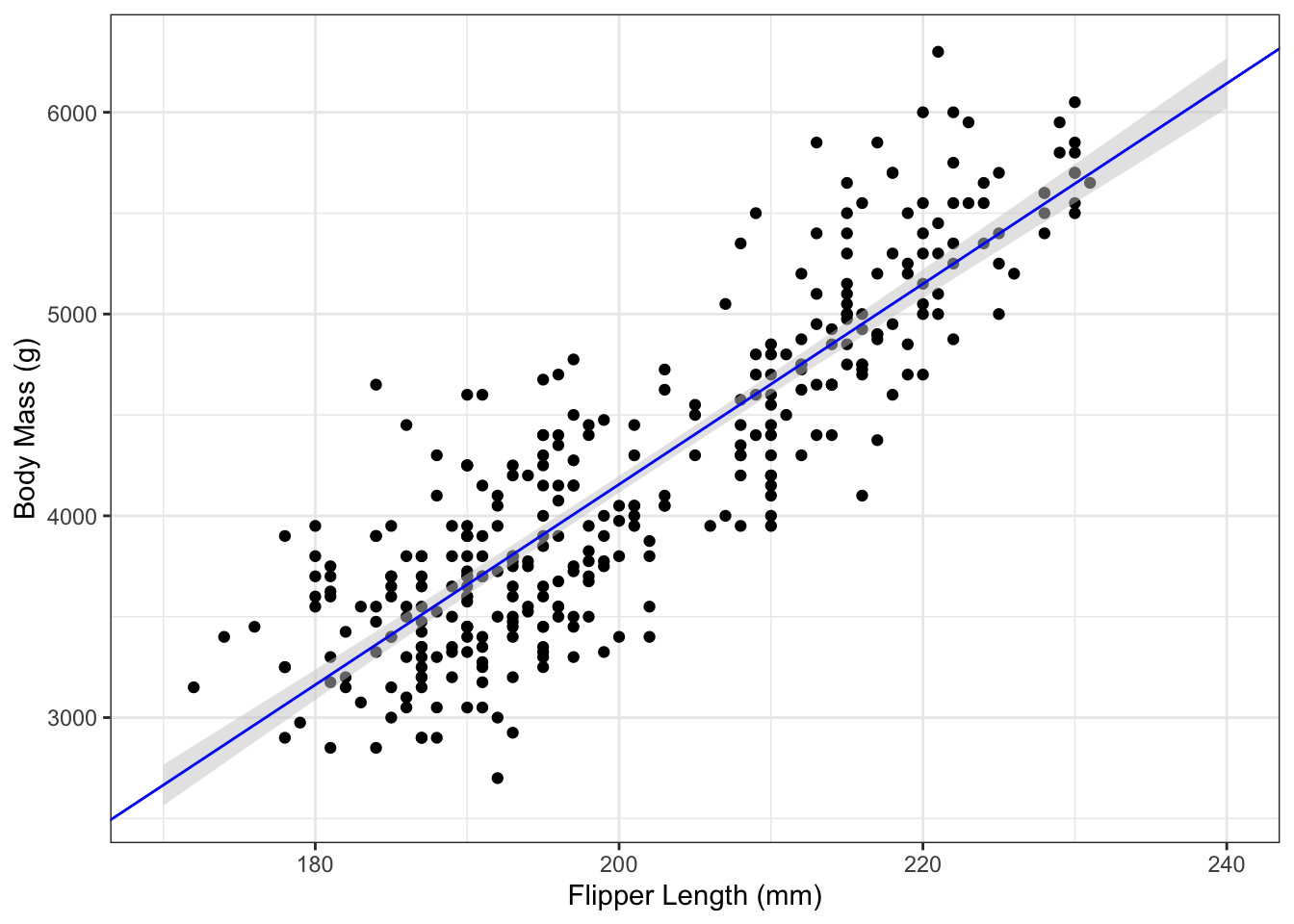
5.2.4.2 Using geom_smooth()
For plotting, it can be much faster to let geom_smooth() do the calculations for you. By calling that function with method="lm" and se=TRUE (the default), we can easily add the fitted regression line and corresponding CI to a plot:
g_penguin+
    geom_smooth(aes(x=flipper_length_mm,
                    y=body_mass_g),
                data=penguins,
                method="lm",
                se=TRUE,
                level=0.95)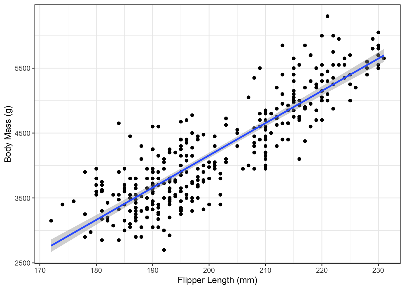
Use the level= argument to geom_smooth() to choose a different confidence level.
5.3 Prediction Intervals
5.3.1 PI for New Observation
Let \(\tilde{Y}_0\) represent a new observation with corresponding predictor value \(x_0\). We predict the value of \(\tilde{Y}_0\) using \(\hat y_0\) from equation (5.2). The difference in mean between the new observation and its prediction is: \[\begin{align*} \E[\tilde{Y}_0 - \hat y_0] &= \E[\tilde{Y}] - \E[\hat{y}_0] \\ &= [\beta_0 + \beta_1x_0] - [\beta_0 + \beta_1x_0] \\ & = 0. \end{align*}\] The variance is: \[\begin{align} \Var(Y_0 - \hat y_0) &= \Var\left( (\beta_0 + \beta_1 x_0 + \epsilon_0) - (\hat\beta_0 + \hat\beta_1x_0) \right)\notag\\ &= \Var\left((\beta_0 + \beta_1 x_0) - (\hat\beta_0 + \hat\beta_1x_0)\right) + \Var(\epsilon_0) \notag\\ &= \sigma^2\left(\frac{1}{n} + \frac{(x_0 - \overline{x})^2}{S_{xx}}\right) + \sigma^2 \notag\\ & = \sigma^2\left(\frac{1}{n} + \frac{(x_0 - \overline{x})^2}{S_{xx}} + 1\right) \tag{5.7} \end{align}\]
Thus, the uncertainty in the new observation is the uncertainty in the estimated mean \(\hat y_0 = \hat\mu_{y|x_0}\) and the uncertainty in a new observation (\(\sigma^2\)).
Using equation (5.7), we can compute a \((1-\alpha)100\%\) prediction interval for a new observation with \(x=x_0\) as:
\[\begin{align} &\Big(\hat y_0 - t_{\alpha/2}\sqrt{\sigma^2\left(1 + \frac{1}{n} + \frac{(x_0 - \overline{x})^2}{S_{xx}}\right)},\notag\\ & \qquad \qquad \hat y_0 + t_{\alpha/2}\sqrt{\sigma^2\left(1 + \frac{1}{n} + \frac{(x_0 - \overline{x})^2}{S_{xx}}\right)} \Big) \tag{5.8} \end{align}\]
A prediction interval is a random interval that, when the model is correct, has a \((1-\alpha)\) probability of containing a new observation that has \(x_0\) as its predictor value.
Heuristically, you can think of a prediction interval as similar to a confidence interval but for an observation, not a parameter. Accordingly, a prediction interval will always be larger than the corresponding confidence interval.
5.3.2 Calculating a PI
As with confidence intervals, we can compute prediction intervals either directly form the formula or using the predict() command.
5.3.2.1 “By Hand”
Creating a prediction interval using the formula (5.8) uses many of the same values as calculating a confidence interval for the mean. If we have already computed \(\widehat{se}(\mu_{y|x_o})\) as seMuHat, then calculating the prediction interval can be done as:
sePred <- sqrt(seMuHat^2 + summary(penguin_lm)$sigma^2)
yhat_PI <- c(muhat - qt(.975, n-2)*sePred, muhat + qt(.975, n-2)*sePred)
yhat_PI
## (Intercept) (Intercept)
## 3379.612 4932.9515.3.2.2 Using predict()
Alternatively, setting interval="prediction" inside predict() will compute the prediction intervals automatically from the model fit:
## fit lwr upr
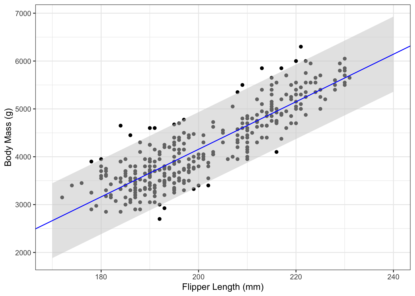
## 1 4156.282 3379.612 4932.951Plotting the prediction interval is also analogous to the confidence interval, except that it can’t be done automatically using geom_smooth(). Instead, we follow the “by hand” approach and make prediction intervals for a sequence and add them to a plot:
body_mass_pi <- predict(penguin_lm,
        newdata=flipper_length_pred_df,
        interval="prediction",
        level=0.95)
body_mass_pi_df <- data.frame(body_mass_pi,
                              flipper_length_pred_df)
g_penguin +
    geom_ribbon(aes(x=flipper_length_mm,
                    ymax=upr,
                    ymin=lwr),
                data=body_mass_pi_df,
                fill="grey80",
                alpha=0.5) +
  geom_abline(aes(slope=coef(penguin_lm)[2],
                  intercept=coef(penguin_lm)[1]), col="blue")