Chapter 13 Unusual Observations

\(\newcommand{\E}{\mathrm{E}}\) \(\newcommand{\Var}{\mathrm{Var}}\) \(\newcommand{\bme}{\mathbf{e}}\) \(\newcommand{\bmx}{\mathbf{x}}\) \(\newcommand{\bmH}{\mathbf{H}}\) \(\newcommand{\bmI}{\mathbf{I}}\) \(\newcommand{\bmX}{\mathbf{X}}\) \(\newcommand{\bmy}{\mathbf{y}}\) \(\newcommand{\bmY}{\mathbf{Y}}\) \(\newcommand{\bmbeta}{\boldsymbol{\beta}}\) \(\newcommand{\bmepsilon}{\boldsymbol{\epsilon}}\) \(\newcommand{\bmmu}{\boldsymbol{\mu}}\) \(\newcommand{\bmSigma}{\boldsymbol{\Sigma}}\) \(\newcommand{\XtX}{\bmX^\mT\bmX}\) \(\newcommand{\mT}{\mathsf{T}}\) \(\newcommand{\XtXinv}{(\bmX^\mT\bmX)^{-1}}\)

The previous chapter focused on how to identify violations of overall model assumptions. But even when there is no evidence of violations of the model assumptions for the full dataset, there can still be individual observations that are atypical.

An observation might be an outlier, in which is notably different from the vast majority of the rest of the data. An outlier observation is not necessarily a problem–but it should be investigated to confirm that it is a plausible value and assess the magnitude of impact it has on the model fit. It’s important o remember that an outlier is not necessarily a problem–but is something that should be investigated.

Leverage and influence are two ways for quantifying how “unusual” an observation is.

13.1 Leverage

A high leverage point is a point that has an unusual combination of predictor variable values. In simple linear regression, this means simply that its value of \(x_i\) is much larger or much smaller than the rest of the data. In multiple linear regression, it might be that one or more of the predictor variables has an extreme value. However, a point can also have high leverage if the combination of predictor variables is unusual.

Figure 13.1 shows a high leverage point in the upper right quadrant. Its \(x\) value of 6 is well outside the range of the other points, which are between 0 and 3.

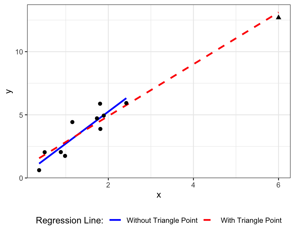
Figure 13.1: The triangle point in the upper left has high leverage, due to its extreme value of \(x\) relative to the other points. The dashed blue line shows the SLR line with this point, the red line is the SLR line with the point included.

13.1.1 Impact of high leverage points

High leverage points can dramatically impact standard errors and measures of model fit (e.g., \(R^2\)). High leverage points can, but do not necessarily, have a large effect on the values of \(\hat\bmbeta\)–that impact is quantified by influence (Section 13.2 below).

Because of their extreme \(x\) values, high leverage points can increase the value of \(S_{xx}\) (in SLR) and \(\bmX^\mT\bmX\) (in MLR) by expanding the amount of variation in the predictor variables. This can lead to smaller values of \(1/S_{xx}\) and \((\bmX^\mT\bmX)^{-1}\), which would result in smaller standard errors.

In situations like Figure 13.1, a high leverage point can inflate \(R^2\). The triangle point does not dramatically affect the estimated regression line, but it does result in a much larger value of \(SS_{tot}\) and \(SS_{reg}\).

Example 13.1 In the data in Figure 13.1, when the high leverage point is not included, \(R^2 = 0.82\) and \(\widehat{se}(\hat\beta_1) = 0.41\). When the high leverage point is included, \(R^2 = 0.94\) and \(\widehat{se}(\hat\beta_1) = 0.18\).

13.1.2 Quantifying Leverage

Leverage can be quantified by the diagonal elements in the hat matrix (\(\bmH = \bmX(\bmX^\mT\bmX)^{-1}\bmX^\mT\)). Recall that the hat matrix controls how much each observation impacts fitted values:

\[\hat\bmy = \bmH\bmy \quad \Rightarrow \quad \hat y_1 = h_{11}y_1 + h_{12}y_2 + \dots h_{1n}y_n\]

The value of \(h_{ij}\) is the amount of weight applied to the \(j\)th observation when predicting the \(i\)th response. The larger the value of \(h_{ii}\) is, the more weight that observation has on its own prediction. Points near the edge of “\(x\)-space” will have large \(h_{ii}\) values, and so the value of \(h_{ii}\) can be used to quantify the leverage of a point.

In R, the values of \(h_{ii}\) can be calculated using the hatvalues() command.

13.2 Influence

An influential point is a point that substantially impacts the regression coefficients. this means the point needs to have an unusually value of the response variable. Influential points can be high leverage points, but points that do not have high leverage can still be influential.

Figure 13.2 shows the impact an influential point can have. When the triangle point is included, the regression line is somewhat flat (red dashed line). But when point is excluded, the regression line is much steeper (blue solid line).

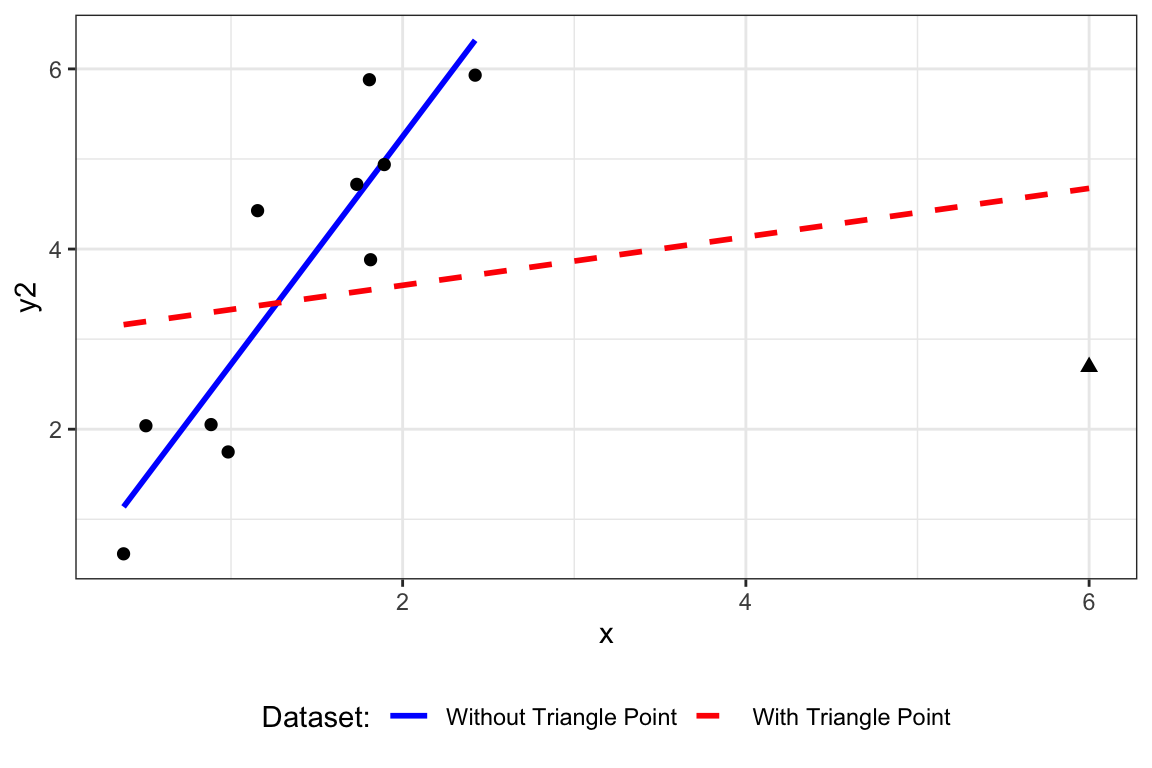
Figure 13.2: Illustration of an influential point (represented by triangle).

13.2.1 Quantifying Influence

Influence can be quantified by comparing how much the model changes when you leave out a data point. These statistics are commonly called “deletion diagnostics”.

Let \(\hat\bmbeta_{(i)}\) denote the OLS estimator when the \(i\)th observation is removed. Let \(\hat\bmy_{(i)}\) denote fitted values using \(\hat\bmbeta_{(i)}\). Deletion diagnostics quantify (i) how \(\hat\bmbeta_{(i)}\) compares to \(\hat\bmbeta\) or (ii) how \(\hat\bmy\) compares to \(\hat\bmy_{(i)}\).

13.2.2 Cook’s D

Cook’s D measures the squared difference between \(\hat\bmbeta\) and \(\hat\bmbeta_{(i)}\), scaled by the locations in `X-space’. This is equivalent to the squared distance that the vector of fitted values changes when you calculate \(\hat\beta\) without the \(i\)th observation. Cook’s D is calculated for each observation.

\[\begin{align*} D_i & = \frac{(\hat\bmbeta_{(i)} - \hat\bmbeta)^\mT(\bmX^\mT\bmX)(\hat\bmbeta_{(i)} - \hat\bmbeta)}{p\hat\sigma^2}\\ & = \frac{(\hat\bmy_{(i)} - \hat\bmy)^\mT(\hat\bmy_{(i)} - \hat\bmy)}{p\hat\sigma^2} \end{align*}\]

In R, Cook’s D can be calculated using the function cooks.distance().

13.2.3 \(DFBETAS\)

A similar statistic is the ‘DF-Beta’, which measures how much \(\hat\beta_j\) changes when the \(i\)th observation is removed. This is commonly calculated on a standardized scale (hence the \(S\) in \(DFBETAS\)).

\[DFBETAS_{j,i} = \frac{\hat\beta_j - \hat\beta_{j(i)}}{\sqrt{\hat\sigma^2_{(i)}((\bmX^\mT\bmX)^{-1})_{jj}}}\]

Unlike Cook’s D, \(DFBETAS\) are calculated for each parameter-observation combination (which is why it is indexed by \(i\) and \(j\)). \(DFBETAS\) tells you which coefficients are most impacted by which observations. This provides an additional level of detail to narrow down how a point is influential.

In R, use the function dfbetas() (note this is not dfbeta()).

13.3 Influence Measures in R

The individual measures of leverage and influence can be calculated as described above, but R also provides a convenient method for computing them all. The function influence.measures() provides all three measures and automatically flags what it thinks are influential values.

13.4 What to do?

If we identify high leverage or influential observations, what should we do?

It’s best to investigate the point, if possible. In large datasets, this may be unfeasible, however. If the point is a data error, it should be corrected or if necessary discarded (and this removal reported). But if the point is a valid observation, it should not be removed simply because it is influential. Alternative models that are more robust to outlying values could be explored.