Chapter 17 Model Selection for Association
\(\newcommand{\E}{\mathrm{E}}\) \(\newcommand{\Var}{\mathrm{Var}}\) \(\newcommand{\bmx}{\mathbf{x}}\) \(\newcommand{\bmH}{\mathbf{H}}\) \(\newcommand{\bmI}{\mathbf{I}}\) \(\newcommand{\bmX}{\mathbf{X}}\) \(\newcommand{\bmy}{\mathbf{y}}\) \(\newcommand{\bmY}{\mathbf{Y}}\) \(\newcommand{\bmbeta}{\boldsymbol{\beta}}\) \(\newcommand{\bmepsilon}{\boldsymbol{\epsilon}}\) \(\newcommand{\bmmu}{\boldsymbol{\mu}}\) \(\newcommand{\bmSigma}{\boldsymbol{\Sigma}}\) \(\newcommand{\XtX}{\bmX^\mT\bmX}\) \(\newcommand{\mT}{\mathsf{T}}\) \(\newcommand{\XtXinv}{(\bmX^\mT\bmX)^{-1}}\)
Acknowledgment: Some of the information in this section was based upon ideas from Scott Emerson and Barbara McKnight.
17.1 Model Misspecification – Mathematical consequences
Suppose we have \(\bmX = \begin{bmatrix} \bmX_q & \bmX_r \end{bmatrix}\) and \(\bmbeta = \begin{bmatrix} \bmbeta_q \\ \bmbeta_r \end{bmatrix}\). Assume the true regression model is: \[\bmy = \bmX\bmbeta + \bmepsilon = \bmX_q\bmbeta_q + \bmX_r\bmbeta_r + \bmepsilon\] with the usual assumptions of \(\E[\bmepsilon] = 0\) and \(\Var(\bmepsilon) = \sigma^2 \bmI\).
17.1.1 Correct model
Suppose we fit the correct model
- Model we fit is: \(\bmy = \bmX_q\bmbeta_q + \bmX_r\bmbeta_r + \bmepsilon\)
- OLS estimator is: \[\hat\bmbeta^* = (\bmX^\mT\bmX)^{-1}\bmX^\mT\bmy\]
- \(\hat\bmbeta\) is unbiased: \[\E[\hat\bmbeta] = (\bmX^\mT\bmX)^{-1}\bmX^\mT\E[\bmy] =(\bmX^\mT\bmX)^{-1}\bmX^\mT(\bmX\bmbeta) = \bmbeta\]
17.1.2 Not including all variables
What happens if we fit model only using \(\bmX_q\) (leaving out the \(\bmX_r\) variables)?
- Model we fit is \(\bmy = \bmX_q\bmbeta_q + \bmepsilon\)
- OLS estimator is: \[\hat\bmbeta_q = (\bmX_q^\mT\bmX_q)^{-1}\bmX_q^\mT\bmy\]
- Expected value of \(\hat\bmbeta_q\) is:
- This means \(\hat\bmbeta_q\) is biased, unless \(\bmbeta_r = \mathbf{0}\) or \(\bmX_q^\mT\bmX_r = \mathbf{0}\) (predictors are uncorrelated).
- Size and direction of bias depends on \(\bmbeta_r\) and correlation between variables.
- It can be shown that \(\hat\sigma^2\) is biased high.
Key Result: Not including necessary variables can bias our results.
17.1.3 Including too many variables
What happens if we include \(\bmX_q\), \(\bmX_r\), and \(\bmX_s\)?
- Model with fit is: \(\bmy = \bmX_q\bmbeta_q + \bmX_r\bmbeta_r + \bmX_s\bmbeta_s + \bmepsilon = \bmX^*\bmbeta^* + \bmepsilon\)
- OLS estimator is: \[\hat\bmbeta^* = (\begin{bmatrix}\bmX & \bmX_s\end{bmatrix}^\mT\begin{bmatrix}\bmX & \bmX_s\end{bmatrix})^{-1}\begin{bmatrix}\bmX & \bmX_s\end{bmatrix}^\mT\bmy\]
- Expected value of \(\hat\bmbeta^*\) is:
- Our estimate of \(\bmbeta\) is unbiased!
- It can be shown that \(\Var(\hat\bmbeta)\) will increase when extraneous variables are added.
This result indicators that adding extra variables does not bias our results, but can increase the variances of \(\hat\bmbeta\) (and thus reduce power). However, this is under a strict mathematical scenario in which the additional variables are uncorrelated with the response. In practice, adding extra variables can lead to bias because of collider bias (see Section ??).
17.2 Confounding, Colliders, and DAGs
17.2.1 Confounders
Confounding is the distortion of a predictor-outcome relationship due to an additional variable(s) and its relationship to the predictor and the outcome. Heuristically, it is a variable that we need to account for, otherwise we can obtain the “wrong” result.
A variable (\(C\)) is a confounder of the relationship between predictor of interest (\(X\)) and outcome (\(Y\)) if both of the following are true:
- \(C\) is causally related to the outcome \(Y\) in the population
- \(C\) is causally related to the predictor of interest \(X\)
It is not enough that a variable is correlated with both \(X\) and \(Y\). The direction of causality must go from the confounder to \(X\) and \(Y\).
17.2.2 Directed Acyclic Graphs (DAGs)
To help think through whether or not a variable is a confounder, it can be helpful to draw a schematic of the relevant causal relationships. This can be done through a directed acyclic graph, commonly abbreviated as a “DAG”.
Note that in this context, a “graph” is not a plot of data, but rather a set of points, called nodes, connected by arrows. The outcome variable, predictor of interest and other variables are the nodes. An arrow between two nodes denotes a causal relationship from one variable to another. The adjective “acyclic” means that a DAG has no closed loops.
DAGs generally show just the existence of a relationship, not its strength or magnitude. And nodes not connected are presumed to have no causal relationship
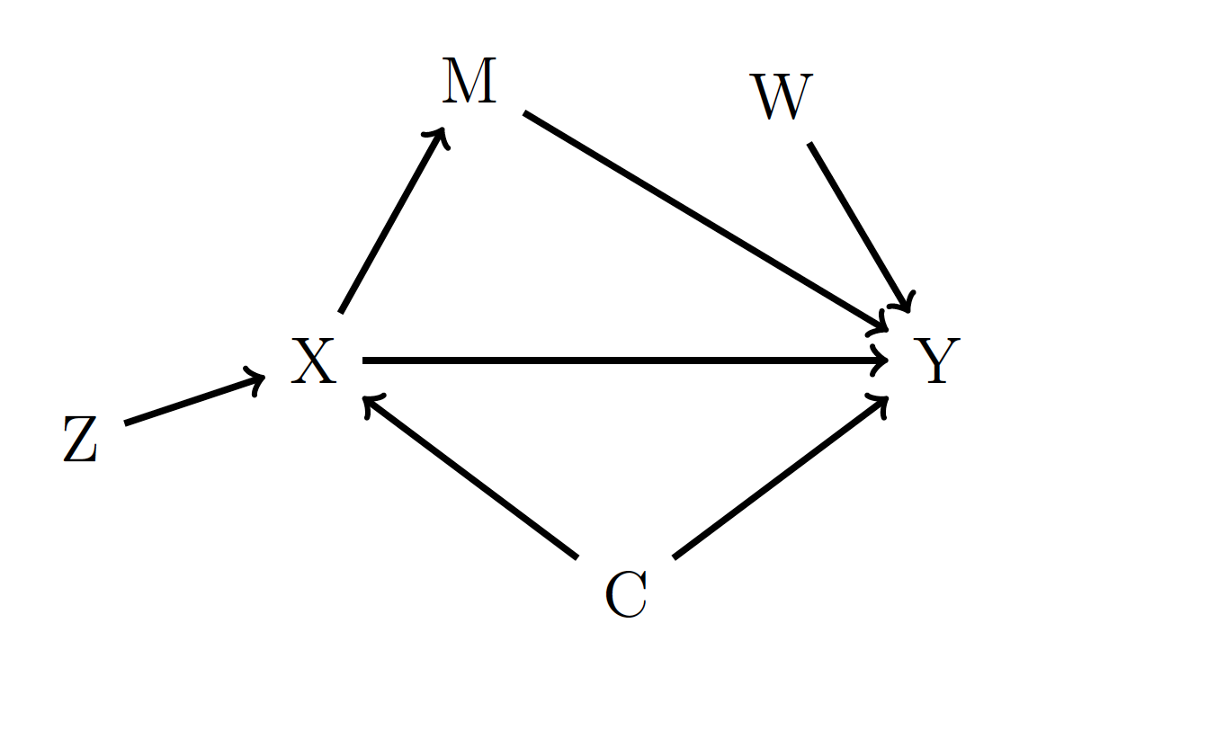
Figure 17.1: An example DAG.
In Figure 17.1, the variable \(C\) is a confounder since it has arrows going from it to both \(X\) and \(Y\). Variable \(M\) is not a confounder. Instead, \(M\) is a mediator, since it lies on a pathway from \(X\) to \(Y\). Variables \(Z\) and \(W\) are neither confounders nor mediators.
17.2.3 Accounting for Confounders
Confounding can have a drastic impact on our results. If ignored, it can lead to completely wrong conclusions. To account for confounders, we adjust for them in the regression model. And when we do this, we should always interpret your results in the context of what is in the model.
17.2.4 Confounding Example: FEV in Children
Consider the question: Is there a relationship between smoking and lung function in children? To answer this, we use data collected from a sample of children. Our outcome variable is forced expiratory volume (FEV), which is a measure of lung function. Higher values of FEV indicate greater lung capacity and better lung health. The predictor of interest for this question is whether or not the child smokes cigarettes. (These data were collected before the invention of vaping devices).
In our sample, these two quantities are stored in the variables fev and smoke, respectively. The smoke variable is coded so that 1 represents a child that smokes and 0 represents a child that does not smoke.
Figure 17.2 shows the distributions of FEV values by the two smoking groups.
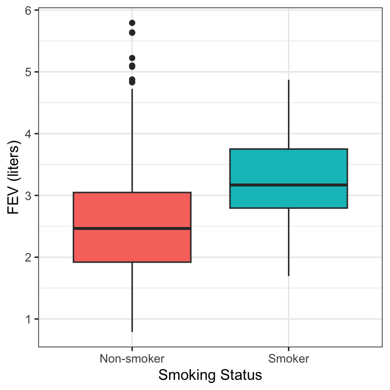
Figure 17.2: Boxplots of FEV by smoking status.
If we fit a simple linear regression model to these data, we obtain the following output:
## # A tibble: 2 × 7
##   term        estimate std.error statistic   p.value conf.low conf.high
##   <chr>          <dbl>     <dbl>     <dbl>     <dbl>    <dbl>     <dbl>
## 1 (Intercept)    2.57     0.0347     74.0  1.49e-319    2.50      2.63
## 2 smoke          0.711    0.110       6.46 1.99e- 10    0.495     0.927
From this model, we would conclude: Children who smoke have on average a 0.71 L greater FEV (95% CI: 0.50, 0.93) than children who do not smoke (\(p<0.0001\)).
However, this result seems to go against our well-founded intuition that smoking should not improve health. So what’s going on here? Figure 17.3 shows the data, but now incorporating information on each child’s age. From the plot, we can see that:
- Older children have higher FEV
- Older children are more likely to be smokers
In other words, age confounds the relationship between smoking status and FEV. This is represented in the DAG in Figure 17.4.
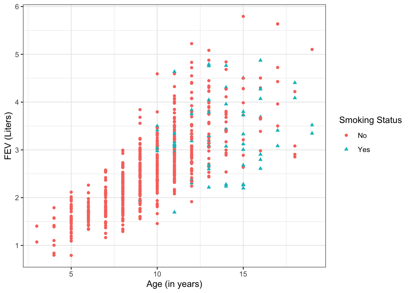
Figure 17.3: Scatterplot of FEV by age.
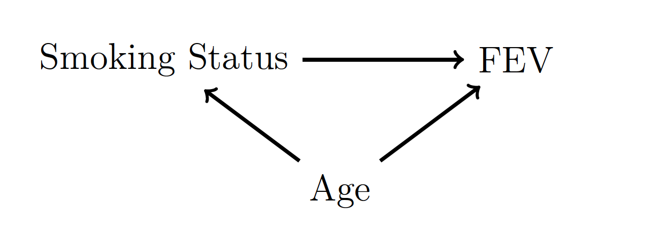
Figure 17.4: A DAG for the FEV data.
Since we have now identified age as a confounder, let’s fit model that also adjusts for age. We obtain the results:
## # A tibble: 3 × 7
##   term        estimate std.error statistic   p.value conf.low conf.high
##   <chr>          <dbl>     <dbl>     <dbl>     <dbl>    <dbl>     <dbl>
## 1 (Intercept)    0.367   0.0814       4.51 7.65e-  6    0.207    0.527
## 2 smoke         -0.209   0.0807      -2.59 9.86e-  3   -0.368   -0.0504
## 3 age            0.231   0.00818     28.2  8.28e-115    0.215    0.247
From this model, we would conclude: Children who smoke have on average a 0.21 L lower FEV (95% CI: -0.37, -0.05) than children of the same age who do not smoke (\(p<0.0001\)).
This shows how by adjusting for the confounder in the MLR model, we can correctly estimate the relationship between smoking and FEV.
17.2.5 Confounding & Randomized Experiments
Confounding is one of the main reasons why randomized experiments so popular. In a randomized experiment, experimental units (rats, trees, people, etc.) are randomly assigned to a treatment condition (food, fertilizer, drug, etc.). The difference in outcome is compared between the different treatment groups. By randomly assigning the treatment conditions, there is no relationship between the treatment condition and any other variables. This means that there is no confounding!
17.2.6 Colliders
Colliders are variables that are downstream of both the predictor of interest and the outcome variable. In a DAG, colliders occupy a similar position to confounders, except that the arrows are pointing in the reverse direction. If colliders are included in a model, then they can introduce spurious correlations and results. This is why drawing a DAG is an important part of model selection. Adding extra variables is not always harmless, since if the variable is a collider it will adversely impact the inference.
17.3 Confirmatory v. Exploratory
17.3.1 Association Study Goals
In studies of association, the goal is to estimate the potential relationship between a predictor and an outcome
- Inference about a quantity (usually \(\beta\)) that summarizes the relationship between predictor and outcome is target, as opposed to accuracy in predicting \(y\)
- Want to limit bias from confounding
- Want high power for detecting an association, if it exists
- Study may be confirmatory or exploratory
17.3.2 Confirmatory Analyses
A confirmatory analysis attempts to answer the scientific question the study was designed to address
- The analysis is hypothesis testing
- Interpretation can be strong
- Analysis must follow a detailed protocol designed before data were collected to protect the interpretation of the \(p\)-value.
- Ex: The statistical analysis plan for all U.S. clinical trials must be published before recruitment begins.
- Variables included in the model and tests performed cannot depend on features of the data that were collected
- Cannot change your model based on what you see in the data you collect
- Protects against overfitting and preserves Type I error rate
- Failure to be strict about the analysis plan is a major factor in the large number of contradictory published results
17.3.3 Exploratory Analyses
An exploratory analysis uses already collected data to explore additional relationships between the outcome and other measured factors
- The analysis is hypothesis generating
- Interpretations should be cautious
- The general analysis plan should be established first, but
- The form of variables in the model (e.g. splines, cut points for categories) may depend on what is found in the data
- The variables chosen for the model and the presence of interactions may depend on what is found in the data
- Exploratory analyses can be basis for future studies, but do not provide definitive evidence
17.3.4 Model Selection Process – Confirmatory Analysis
For a confirmatory analysis:
- State the question of interest and hypothesis
- Identify relevant causal relationships and confounding variables
- Specify the model
- Specify the form of the predictor of interest
- Specify the forms of the adjustment variables
- Specify the hypothesis test that you will conduct
- Collect data.
- Fit the pre-specified model and conduct the pre-specified hypothesis test.
- Present the results
17.3.5 Model Selection Process – Exploratory Analysis
For an exploratory analysis:
- State the question of interest and hypothesis
- Identify relevant causal relationships and confounding variables
- Perform a descriptive analysis of the data
- Specify the model
- Specify the form of the predictor of interest
- Specify the forms of the adjustment variables
- Fit the model.
- Develop hypotheses about possible changes to the model.
- Assess the evidence for changes to the model form, using hypothesis tests
- Identify model(s) that fit data and science well
- Present the results as exploratory
17.3.6 Identifying a Statistical Model
- Collect your data and choose your statistical model based on what question you want to answer.
- Do not choose the question to answer just based on a statistical model or because you have a certain type of data.
- Better to have an imprecise answer to the right question than a precise answer to the wrong question
- Do not ignore confounding for the sake of improving power, since this will lead to biased estimates
- “Validity before precision”
- Variable selection should be based upon understanding of science and causal relationships (e.g. DAGs), not statistical tests of relationships in the data.
17.4 Variable Selection
17.4.1 What not to do
Many “automated” methods for variable/model selection exist
- Forwards selection
- Backwards elimination
- Minimizing AIC/BIC
While rule-based and simple to implement, these are not appropriate methods to use for selecting a model to test an association.
Statistical issues can impact model estimates
- Outliers, high-leverage points, and influential observations can have out-sized impact on model fit
- Including multiple correlated adjustment variables can inflate standard errors and reduce power (multicollinearity)
These are statistical issues that should be considered in overall assessment and interpretation of your model. But they should not drive variable selection.
17.4.2 Predictor of Interest
Confirmatory Analysis
- Choose form (e.g. linear, log, quadratic, etc.) consistent with the prior hypothesis
Exploratory Analysis
- Include all relevant exposure variables in the model
- Explore what form fits best
- Unordered categorical?
- Linear, Logarithmic, Quadratic?
- What is best category size? (e.g. 2-year or 5-year groups)
17.4.3 Adjustment Variables
Confirmatory Analysis
- Include variables if your prior hypothesis is that they are confounders
- Form should be as flexible as possible, to reduce residual confounding
- Unordered indicators for categorical variables
- Spline representations of continuous variables (often 3 df is enough, but not always)
- Interactions between confounders, if there is a priori reason to hypothesize such a relationship
Exploratory Analysis
- Develop list of scientifically plausible confounders (i.e. draw a DAG)
- Include plausible confounders in the model
- Explore the impact of different forms of the variables
- Linear v. spline for continuous
- Variations in cut point of categories
- Interactions
17.4.4 Things to Consider
When developing DAGs and identifying confounders for inclusion in the model, some points to keep in mind:
- Are two plausible confounders meaningfully different?
- Ex: Employment status and personal income
- Sample size
- With large \(n\), can disentangle differences between related variables
- Small sample sizes make estimating many parameters difficult
- If \(n=100\), don’t include splines with 50 df or a variable with 30 categories!
- However, sample size alone should not determine your model!
- Always include lower-order terms
- If including interaction, include main effects
- If including quadratic term, include linear term
- Interactions
- Interactions are often hard to estimate unless very strong
- Confounding can depend greatly on the presence of interactions
- Interactions often subject of exploratory analyses, but not as common as primary question for a confirmatory analysis
- Parsimony
- Traditionally, parsimonious models have been preferred, since they are easier to interpret
- Modern datasets and questions are typically too complex for simple models to be appropriate
- A model can be scientifically parsimonious but still statistically complex
17.5 Exercises
Exercise 17.1 Does ice cream sales cause shark bites?
- Predictor of Interest: Ice Cream Sales
- Outcome: Number of shark bites
- We also know:
- Ice cream sales are higher during warm weather
- More people are at the beach during warm weather
Draw a DAG representing these relationships.
Exercise 17.2 Vaccine trials for COVID-19 compare rates of infection in treatment and placebo groups, without adjusting for anything else. Why is there no confounding?