Chapter 2 Simple Linear Regression

\newcommand{\E}{\mathrm{E}} \newcommand{\Var}{\mathrm{Var}}

2.1 The Simple Linear Regression (SLR) Model

2.1.1 Goal of SLR

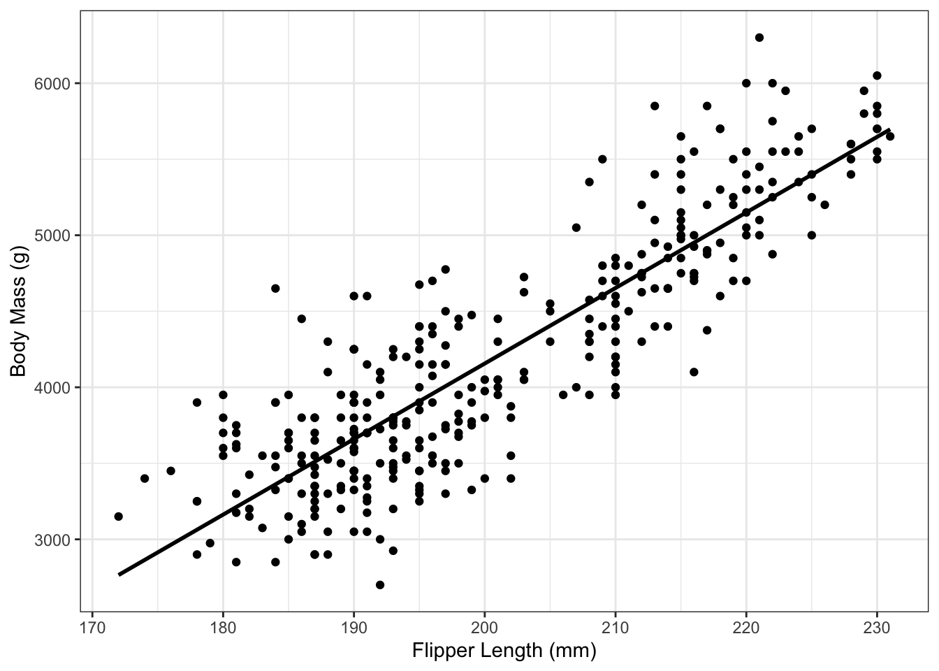
In simple linear regression (SLR), our goal is to find the best-fitting straight line, commonly called the regression line, through a set of paired (x, y) data. The line should go through the “middle” of the data and represent the “average” trend in the outcome variable as a function of the predictor variable. Throughout this chapter and the next, we will look at how to more precisely define what the line represents, how to interpret it in context, and how to estimate it.

Example 2.1 In Example 1.1, we introduced data on penguin flipper length and body mass. The following plot shows the data and the corresponding linear regression line:

2.1.2 Theoretical SLR model

The general form for the equation of a line includes a slope and intercept. For regression, we use that form but also add an error term that accounts for random deviation around the line.

There are two complimentary ways to think about the SLR model. The first is as a theoretical mathematical model for random variables and the second is as a calculated line for specific dataset. Here we first introduce the theoretical model. The calculated line for a specific dataset is discussed in Section 2.2. Later chapters will present both together.

Let i be an index for each observation (penguins, people, units, etc.) The theoretical equation for the Simple Linear Regression (SLR) model is:

\begin{equation} Y_i = \beta_0 + \beta_1x_i + \epsilon_i \tag{2.1} \end{equation}

where:

• Y_i is a random variable representing the outcome variable (e.g. body mass)

• x_i is a fixed predictor variable (e.g., flipper length)

• \beta_0 is a parameter representing the intercept

• \beta_1 is a parameter representing the slope

• \epsilon_i is a random variable representing variation (the “error” in the model)

These five elements can be categorized as three different kinds of quantities:

• Random variables (Y_i and \epsilon_i): Random quantities that are not directly observed. For a given dataset, the corresponding observed values will be denoted y_i and e_i (See Section 2.2)
• Parameters (\beta_0 and \beta_1): Numbers that are fixed but unknown. These values are the same for all observations in the model. Estimating the values of these parameters (the topic of Section 3) is the basic task in “fitting” a regression model.
• Observed data (x_i): Values that are fixed and known. Each observation can have a different value of x_i, or there could be as few as only two distinct values for x_i. Even though these might vary between datasets, the SLR model considers them fixed. SLR refers specifically to settings where there is only one predictor variable. In Chapter 8 we will extend this to multiple predictor variables.

2.1.3 SLR Model Assumptions

The assumptions corresponding to the SLR model (equation (2.1)) are:

1. \E[\epsilon_i] = 0
   • The error terms have mean zero. This allows the \epsilon_i to account for variability above and below the line.
2. \Var[\epsilon_i] = \sigma^2
   • The error terms have constant variance. (If the variance was different for each observation, then \Var[\epsilon_i] = \sigma_i^2.)
3. \epsilon_i are uncorrelated
   • Each observation gives you new information. This usually means that each observation is independent.

For now, the key assumption is E[\epsilon_i] = 0. Importantly, we do not require an assumption about normality of the error term. We will discuss these assumptions in detail, including what happens when they are violated and how to check if they are satisfied, in Chapter 12.

2.2 Random Variables v. Data

The theoretical SLR model (2.1) is an equation for the random variables Y_i. In practice, we observed data y_i and estimate a line that has an estimated slope and intercept.

In other words, real data are not generated from the theoretical model Y_i = \beta_0 + \beta_1x_i + \epsilon_i But for a dataset with specific values (x_i, y_i), we can use the theoretical model to describe the data:

\begin{equation} y_i = \hat\beta_0 + \hat\beta_1x_i + e_i \tag{2.2} \end{equation}

In equation (2.2):

• y_i is the observed value of the outcome for observation i
• e_i is the residual value corresponding to observation i
• \hat\beta_0 is the estimated intercept for the regression line
• \hat\beta_1 is the estimated slope for the regression line
• x_i is observed value of the predictor variable for observation i

The “hats” in \hat\beta_0 and \hat\beta_1 indicate that the values are estimates of the true parameter \beta_1 and \beta_0. The difference between the theoretical model and estimated model can be summarized in the following table:

Theoretical/Math World	Real World Data
Y_i = outcome (a random variable)	y_i = outcome (a known number)
x_i = predictor (a known number)	x_i = predictor (a known number)
\epsilon_i= error (a random variable)	e_i = residual (a known number)
\beta_0 = intercept parameter (an unknown number)	\hat\beta_0 = intercept estimate (a calculated number)
\beta_1 = slope parameter (an unknown number)	\hat\beta_1 = slope estimate (a calculated number)

2.3 Parameter Interpretation

2.3.1 Regression Line Equation

A consequence of Assumption 1 (\E[\epsilon_i] = 0) is that the mean of Y_i is a straight line:

\begin{align} \E[Y_i] &= \E[\beta_0 + \beta_1x_i + \epsilon_i] \notag\\ &= \E[\beta_0 + \beta_1x_i] + \E[\epsilon_i]\notag\\ &= \beta_0 + \beta_1x_i + 0 \notag\\ &= \beta_0 + \beta_1x_i \tag{2.3} \end{align}

This allows us to interpret the parameters \beta_0 and \beta_1 in terms of the slope and intercept of the line for the average value of the outcome.

In this section only, we are assuming that \beta_0, \beta_1, and \sigma^2 are known. Starting in Section 3 we will introduce estimates of this parameter and start including “estimated” in interpretations.

2.3.2 Interpreting \beta_1

The \beta_1 parameter represents the slope of the regression line. In other words, \beta_1 is the difference in \E[Y_i] between observations that differ in x_i by one unit.

In almost any data analysis project, an important task is providing an interpretation of the model parameters. When describing the interpretation of \beta_1, it is important to include these key elements:

• An interpretation of \beta_1 as an estimated difference in the average value of the outcome variable
  • For linear regression, “difference in average” is the same as “average difference”. You can use either phrase.
• Specify that this is for a 1-unit difference in the predictor variable (x).
• Be cautious about referring to \beta_1 as an “increase” or a “decrease”. Those words imply that an intervention was conducted, in which the value of x was directly modified. This is possible in controlled experiments, but is not the case for observational datasets. To indicate direction, it can be helpful to use words such as “greater”, “lower”, or “higher”.
• Include confidence intervals (see Section 4.8)²
• If appropriate, include information about the conclusion from a hypothesis test (see Section 4.5)³
• Include units for both the outcome and predictor
• If known, include statement about population/context.

Example 2.2 Consider two groups of penguins:

• Penguins that have flipper lengths of 201mm. Call this “Group A”
• Penguins that have flipper lengths of 200mm. Call this “Group B”

Assuming the SLR model (2.1), what is the difference in average body mass between these groups of penguins? To answer this, first write out the regression equation for the mean body mass in each group:

\text{Group A:} \quad \E[Y_A] = \beta_0 + \beta_1*201 \text{Group B:} \quad \E[Y_B] = \beta_0 + \beta_1*200

Then take the difference between them: \begin{align*} \E[Y_A] - \E[Y_B] &= \left(\beta_0 + \beta_1*201 \right) - \left(\beta_0 + \beta_1*200\right)\\ & = 201\beta_1 - 200\beta_1\\ &= \beta_1 \end{align*}

Possible summarizing sentences for \beta_1:

• \beta_1 is the difference in average body mass (in g) for penguins that differ in flipper length by 1 mm.
• The average difference in body mass for penguins that have 1 mm longer flippers is \beta_1 grams.
• The difference in average body mass for penguins that differ in flipper length by one millimeter is \beta_1 grams.

We will expand upon these sentences in Examples 2.8 and 4.7.

2.3.3 Interpreting c\beta_1

Because \beta_1 is the slope of the regression, we can easily interpret multiple of \beta_1, say c\beta_1 for some c \in \mathbb{R}, as differences in the average value of the outcome variable for differences of c units in the predictor variable.

Example 2.3 In Example 2.2, the value 10\beta_1 can be summarized as: the difference in average body mass (in g) for penguins that differ in flipper length by 10 mm.

Example 2.4 In Example 2.2, the value 25\beta_1 can be summarized as: the difference in average body mass (in g) for penguins that differ in flipper length by 2.5 cm.

Interpreting multiples of \beta_1 is closely related to the idea of re-scaling the predictor x, which is covered in Section 7.2.

2.3.4 Interpreting \beta_0

The \beta_0 parameter represents the intercept of the regression line. In other words, \beta_0 is the average value of Y_i (i.e. \E[Y_i]) for observations with an x value of 0. While mathematically useful, \beta_0 might make no practical or scientific sense!

When describing the interpretation of \beta_0, follow all of the same guidelines as for \beta_1 above, with the following exception:

• Interpret it as the average value of the outcome variable (as opposed to a difference in the average value).
• Specify it corresponds to a value of 0 for x, rather than a 1-unit difference in x.

Example 2.5 Consider a third group of penguins:

• Penguins with flipper length of 0 mm. Call this “Group C”

\text{Group C:} \quad \E[Y_C] = \beta_0 + \beta_1*0 = \beta_0

Equivalent interpretation statements for \beta_0 in this context:

• \beta_0 is the average body mass (in g) for penguins that have a flipper length of 0 mm.
• The average body mass for penguins that have 0 mm long flippers is \beta_0 grams.

2.3.5 Interpreting \beta_0 + \beta_1x_i

From Equation (2.3), the points on the regression line can be interpreted as the average value of the outcome variable for units with a particular value of x.

Example 2.6 Consider penguins in Group A (from Example 2.2). In terms of parameters in the simple linear regression mdoel, what is their average body mass?

Since penguins in Group A have flipper lengths of x_i = 200mm, their average body mass is given by:

\E[Y_i | x_i = 200] = \beta_0 + 200\beta_1.

In Section 5, we will see more on how to interpret this value and the difference between estimating a mean and predicting a new observation.

2.3.6 Interpretation of \sigma^2

The parameter \sigma^2 represents the variance of the data around the regression line:

\begin{align*} \Var(Y_i) &= \Var(\beta_0 + \beta_1x_i + \epsilon_i)\\ &= \Var(\beta_0 + \beta_1x_i) + \Var(\epsilon_i)\\ &= 0 + \sigma^2\\ &= \sigma^2 \end{align*}

• A large value of \sigma^2 means that data are more spread out vertically around the line.
• A small value of \sigma^2 means that data are vertically close to the line

The following two plots show simulated data. The left panel has data generated from a model with \sigma^2 = 10 and the right panel data comes from a model with \sigma^2 = 1.

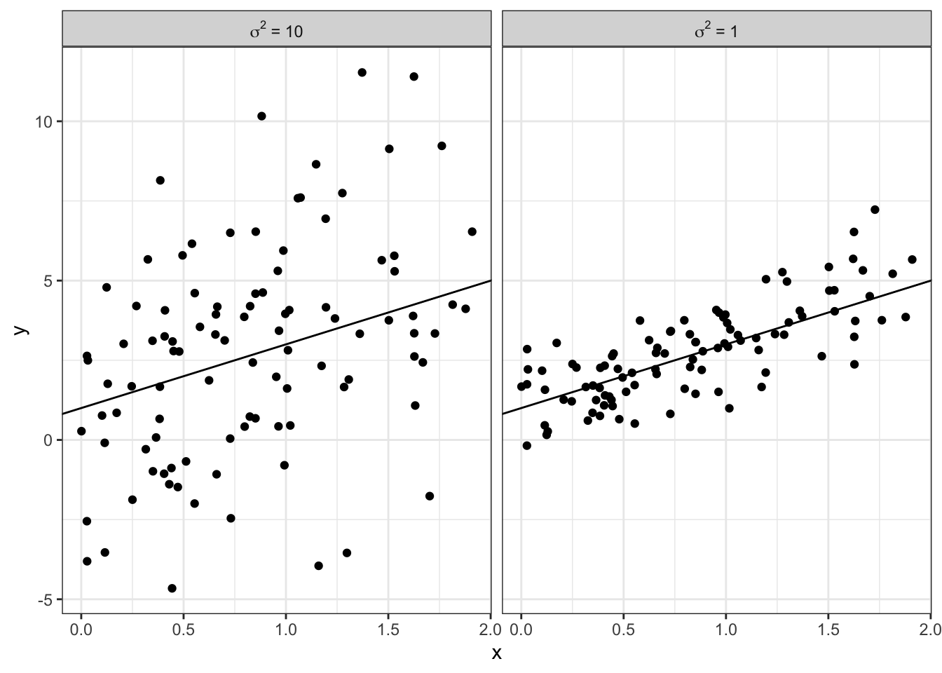
Figure 2.1: Simulated data showing the impact of different values of \sigma^2.

2.3.7 Interpreting \beta_1 with binary x

Although the most common setting of the simple linear regression model is with a continuous predictor variable (such as flipper length), the model can equally be applied when the predictor variable is binary, meaning it takes on two values.

If x_i can take on two values, then instead of a line, the SLR model simply becomes two distinct average values for the two groups. Suppose for one group, x = 0 and for the other group, x=1. A variable defined this was is called an indicator variable since it serves as a binary marker of group membership. The two groups could be anything, such as male/female, home/away, automatic/manual, etc. (We will see how to use indicators for variables with 3 or more categories in Section 11.)

Then the two “lines” for the model are: \begin{align*} \E[Y_i | x_i = 0] &= \beta_0\\ \E[Y_i | x_i = 1] &= \beta_0 + \beta_1*1 = \beta_0 + \beta_1 \end{align*} The average value of the outcome for those with x_i=0 is \beta_0 and the average value of the outcome for those with x_i =1 is \beta_0 + \beta_1. Furthermore, the difference between these values is: \begin{align*} \E[Y_i | x_i = 1] - \E[Y_i | x_i = 0] &= (\beta_0 + \beta_1) - (\beta_0) \\ &= \beta_1 \end{align*} Thus, the interpretations of \beta_0 and \beta_1 are:

• \beta_0 is the average value of Y among observations in the group with x=0
• \beta_1 is the difference in average value of Y between observations with x=1 and those with x=0.

Example 2.7 Consider the penguin data, but now when we model body mass (the outcome) as a function of penguin sex (the predictor variable). Define the indicator variable

\begin{equation} x = \begin{cases} 0 & \text{ if } \texttt{sex} \text{ is } \texttt{"female"} \\ 1 & \text{ if } \texttt{sex} \text{ is } \texttt{"male"} \end{cases}. \tag{2.4} \end{equation} Then in the SLR model Y_i = \beta_0 + \beta_1x_i + \epsilon_i, we have the following interpretations for the regression parameters:

• \beta_0 is the average body mass for female penguins.
• \beta_0 + \beta_1 is the average body mass for male penguins.
• \beta_1 is the difference in body mass between male and female penguins.

2.4 Putting it together: Penguin example

Example 2.8 In the example of penguin flipper length and body mass, the equation for the estimated regression line is: y_i = -5780.8 + 49.7*x_i (We will see how these numbers are calculated in Section 3.) We can interpret the slope of this regression line as follows:

A difference of one mm in flipper length is associated with an estimated difference of 49.7 g greater average body mass among penguins in Antarctica.

Note the key elements in this sentence:

• “average” – Linear regression model tells us about the mean, not a specific observation
• “estimated” – The number 49.7 is an estimate of the true (and unknown) parameter value.
• Units are provided for flipper length and body mass.
• “among penguins in Antarctica” – Context and/or population
• This is observational data, so the relationship is stated as an association, not causation.

Figure 2.2 shows this slope and intercept graphically.

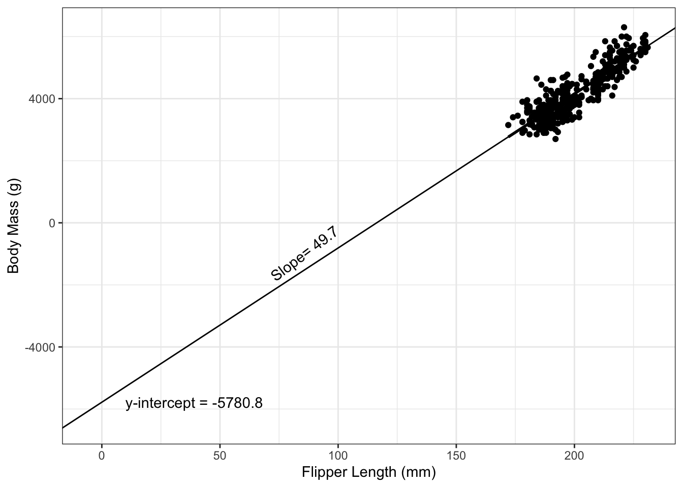
Figure 2.2: Fitted regression line for penguin data.

The residuals for each observation can be calculated as the difference between each data point and its corresponding modeled mean: e_i = y_i - (\hat\beta_0 + \hat\beta_1x_i) Figure 2.3 shows a graphical representation of the residuals e_i.

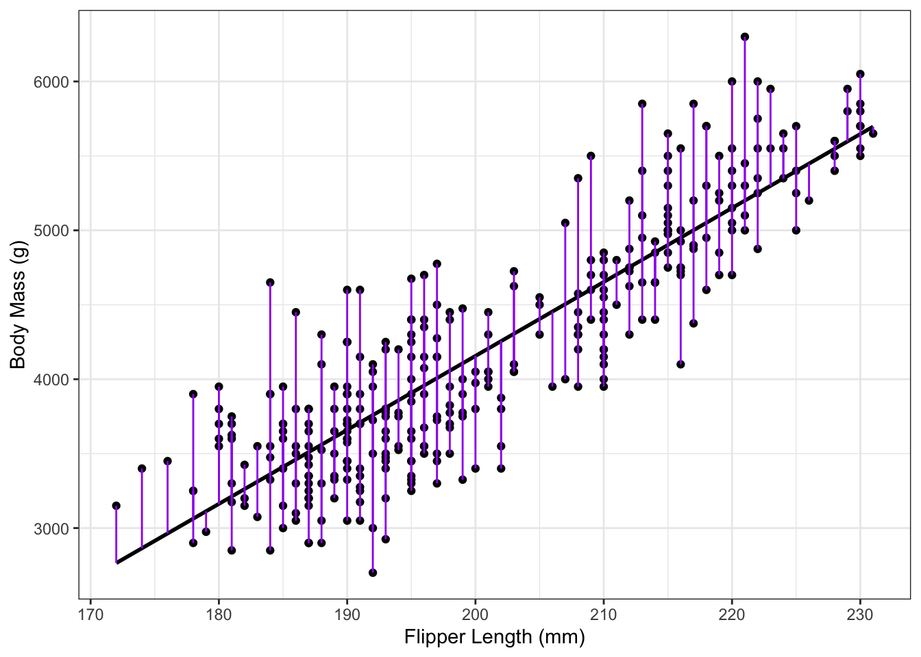
Figure 2.3: Residuals for penguin data.

2.5 Exercises

Exercise 2.1 In the context of Example 2.2, what is an interpretation of 5\beta_1?

Exercise 2.2 In the context of Example 2.5, does the quantity 10\beta_0 make practical sense? If yes, provide an interpretation. If no, explain why not.

Exercise 2.3 Consider a variation of Example 2.2, in which a simple linear regression mdoel is fit with body mass (in g) as the predictor variable and flipper length (in mm) as the outcome. Explain how this switch affects the interpretations of \beta_0, \beta_1, and \sigma^2.

Exercise 2.4 Consider a SLR model with flipper length as the outcome and sex as the predictor, with x defined as in equation (2.4). What are the interpetations of \beta_0 and \beta_1?

Exercise 2.5 In the SLR model of Example 2.7, what is the difference in average body mass between females and male? (Note that the order of the queston is important here).

---

2. The examples in this chapter will skip this for now. This will be added in the examples in Section 4.9↩︎

3. The examples in this chapter will skip this for now. This will be added in the examples in Section 4.9↩︎