Chapter 3 Estimating SLR Parameters
\(\newcommand{\E}{\mathrm{E}}\) \(\newcommand{\Var}{\mathrm{Var}}\)
In Example 2.8, we saw how to interpret the values of estimated slopes and intercepts. But how do we obtain estimates of \(\beta_0\), \(\beta_1\), and \(\sigma^2\)? Ideally, the line should be as close as possible to the data. But for any real-world dataset, the values will not lie directly in a straight line. So how do we define “close enough”?
3.1 Ordinary Least Squares Estimation of Parameters
The standard way is to choose values for \(\beta_0\) and \(\beta_1\) to minimize the sum of squared vertical distances between the observations \(y_i\) and the regression line. We will denote these chosen values as \(\hat\beta_0\) and \(\hat\beta_1\). Minimizing the distance between \(y_i\) and the fitted line \(\hat\beta_0 + \hat\beta_1x_i\) is equivalent to minimizing the sum of squared residuals. Confusingly, this is often called the residual sum of squares and it is defined as4 \[\begin{equation} SS_{Res} = SS_{Res}(\hat\beta_0, \hat\beta_1) = \sum_{i=1}^n e_i^2 = \sum_{i=1}^n \left(y_i - \left(\hat\beta_0 + \hat\beta_1x_i\right)\right)^2 \tag{3.1} \end{equation}\] Estimating \(\hat\beta_0\) and \(\hat\beta_1\) by minimizing \(SS_{Res}\) is called ordinary least squares (OLS) estimation of the SLR parameters. In the rest of this subsection we will explain how to minimize this function mathematically. But in practice this is done by software–so if you just want to know that, skip ahead to Section 3.3.
To find the minimum of the value in (3.1), we can use standard calculus steps for finding a local extrema:
- Find the derivatives of \(SS_{Res}(\hat\beta_0, \hat\beta_1)\) with respect to \(\hat\beta_0\) and \(\hat\beta_1\).
- Set the derivatives equal to zero.
- Solve for the values of \(\hat\beta_0\) and \(\hat\beta_1\)
This procedures yields the “critical point” of \(SS_{Res}(\hat\beta_0, \hat\beta_1)\) (in “\(\beta\)-space”), which we know to be a minimum because \(SS_{Res}(\hat\beta_0, \hat\beta_1)\) is a convex function.
Step 1: Find the two partial derivatives of \(SS_{Res}(\hat\beta_0, \hat\beta_1)\):
\[ \begin{aligned} SS_{Res}(\hat\beta_0, \hat\beta_1) & = \sum_{i=1}^n \left(y_i^2 - 2\hat\beta_0y_i -2\hat\beta_1y_ix_i + \hat\beta_0^2 + 2\hat\beta_0\hat\beta_1x_i + \hat\beta_1^2x_i^2\right)\\ \frac{\partial SS_{Res}}{\partial \hat\beta_0} &= \sum_{i=1}^n \left(-2y_i + 2\hat\beta_0 + 2\hat\beta_1x_i \right) = -2 \sum_{i=1}^n (y_i - \hat\beta_0 - \hat\beta_1x_i)\\ \frac{\partial SS_{Res}}{\partial \hat\beta_1} &= \sum_{i=1}^n \left( -2y_ix_i+ 2\hat\beta_0x_i + 2\hat\beta_1x_i^2\right) = -2 \sum_{i=1}^n (y_i - \hat\beta_0 - \hat\beta_1 x_i) x_i \end{aligned} \]
Step 2: Set them equal to zero: \[\begin{align*} -2 \sum_{i=1}^n (y_i - \hat\beta_0 - \hat\beta_1x_i) &= 0\\ -2 \sum_{i=1}^n (y_i - \hat\beta_0 - \hat\beta_1 x_i) x_i & = 0 \end{align*}\]
and simplify: \[\begin{align} n\hat\beta_0 + \hat\beta_1\sum_{i=1}^n x_i & = \sum_{i=1}^n y_i \tag{3.2} \\ \hat\beta_0 \sum_{i=1}^n x_i + \hat\beta_1\sum_{i=1}^n x_i^2 & = \sum_{i=1}^n x_iy_i \tag{3.3} \end{align}\]
Step 3: Solve for \(\hat\beta_0\) in (3.2): \[\begin{align} n\hat{\beta}_0 + \hat\beta_1 \sum_{i=1}^nx_i = \sum_{i=1}^ny_i \quad \Rightarrow \quad \hat{\beta}_0 & = \frac{1}{n}\sum_{i=1}^ny_i - \hat\beta_1 \frac{1}{n} \sum_{i=1}^nx_i \notag \\ &= \overline{y} - \overline{x}\hat\beta_1 \tag{3.4} \end{align}\]
Plug \(\hat{\beta_0}\) into (3.3) and solve for \(\hat\beta_1\): \[\begin{align*} &\left(\frac{1}{n} \sum_{i=1}^n y_i - \hat\beta_1 \frac{1}{n}\sum_{i=1}^n x_i\right) \sum_{i=1}^nx_i + \hat\beta_1 \sum_{i=1}^n x_i^2 = \sum_{i=1}^n x_iy_i \\ &\left(\sum_{i=1}^n x_i^2 - \frac{1}{n} \left(\sum_{i=1}^n x_i \right)^2 \right)\hat\beta_1 = \sum_{i=1}^n x_iy_i - \frac{1}{n} \sum_{i=1}^n y_i \sum_{i=1}^n x_i \end{align*}\]
\[\begin{align} \hat{\beta}_1 &= \dfrac{\sum_{i=1}^n\limits x_iy_i - \dfrac{1}{n} \sum_{i=1}^n\limits y_i \sum_{i=1}^n\limits x_i }{\sum_{i=1}^n\limits x_i^2 - \dfrac{1}{n} \left(\sum_{i=1}^n\limits x_i \right)^2} \notag \\ &= \dfrac{\dfrac{1}{n}\sum_{i=1}^n\limits x_iy_i - \overline{y}\overline{x} }{\dfrac{1}{n}\sum_{i=1}^n\limits x_i^2 - \overline{x}^2} \tag{3.5} \end{align}\]
Equations (3.4) and (3.5) together give us the formulas for computing both regression parameters estimates. \(\hat\beta_0\) and \(\hat\beta_1\) are the (ordinary) least squares estimators of \(\beta_0\) and \(\beta_1\)
3.2 Understanding \(\hat\beta_1\) with correlation
A common alternative to the form of \(\hat\beta_1\) in (3.5) is to define the following sums-of-squares:
- \(\displaystyle S_{x}^2 = \sum_{i=1}^n x_i^2 - \frac{1}{n} \left(\sum_{i=1}^n x_i \right)^2\)
- \(\displaystyle S_{xy} = \sum_{i=1}^n x_iy_i - \frac{1}{n} \sum_{i=1}^n y_i \sum_{i=1}^n x_i\) \(\qquad\) \(\displaystyle\)
- \(\displaystyle S_{y}^2 = \sum_{i=1}^n y_i^2 - \frac{1}{n} \left(\sum_{i=1}^n y_i \right)^2\)
The sums-of-squares \(S_{x}^2\) and \(S_{y}^2\) represent the total variation in the \(x\)’s and \(y\)’s, respectively. The value of \(S_{xy}\) is the co-variation between the \(x\)’s and the \(y\)’s and takes the same sign as their correlation. In fact, we can show that the Pearson correlation between \(x\) and \(y\) is equal to:
\[r_{xy} = \frac{S_{xy}}{S_xS_y}\]
Using these quantities, an equivalent formula for \(\hat\beta_1\) is \[ \hat\beta_1 = \frac{S_{xy}}{S_{x}^2} = r_{xy}\frac{S_y}{S_x}\] In this form, we can see that the slope of the regression line depends on the correlation betwee \(x\) and \(y\) and the amount variation in each. Importantly, notice that the sign of \(\hat\beta_1\) (i.e., whether it is positive or negative) is the same as the sign of the correlation \(r_{xy}\). Thus, if two variables are positively correlated, their SLR slope will be positive. And if they are negatively correlated, their slope will be negative. We will return to this idea in Section 4.1.
3.3 Fitting SLR models in R
The task of computing \(\hat\beta_0\) and \(\hat\beta_1\) is commonly called “fitting” the model. Although we could explicitly compute the values using equations (3.4) and (3.5), it is much simpler to let R do the computations for us.
3.3.1 OLS estimation in R
The lm() command, which stands for linear model, is used to fit a simple linear regression model in R. (As we will see in Section 8, the same function is used for multiple linear regression, too.) For simple linear regression, there are two key arguments for lm():
- The first argument is an R formula of the form
y ~ x, wherexandyare variable names for the predictor and outcome variables, respectively. - The other key argument is the
data=argument. It should be given adata.frameortibblethat contains thexandyvariables as columns. Although not strictly required, thedataargument is highly recommended. Ifdatais not provided, the values ofxandyare taken from the global environment; this often leads to unintended errors.
Example 3.1 To compute the OLS estimates of \(\beta_0\) and \(\beta_1\) for the penguin data, with flipper length as the predictor and body mass as the outcome, we can use the following code:
Here, we have first loaded the palmerpenguins package so that the penguins data are available in the workspace. In the call to lm(), we have directly supplied the variable names (body_mass_g and flipper_length_mm) in the formula argument, which is unnamed. For the data argument, we have supplied the name of the tibble containing the data. It is good practice to save the output from lm() as an object, which facilitates retrieving additional information from the model.
To see the point estimates, we can simply call the fitted object and it will print the model that was fit and the calculated coefficients:
##
## Call:
## lm(formula = body_mass_g ~ flipper_length_mm, data = penguins)
##
## Coefficients:
##       (Intercept)  flipper_length_mm
##          -5780.83              49.69
To see more information about the model, we can use the summary() command:
##
## Call:
## lm(formula = body_mass_g ~ flipper_length_mm, data = penguins)
##
## Residuals:
##      Min       1Q   Median       3Q      Max
## -1058.80  -259.27   -26.88   247.33  1288.69
##
## Coefficients:
##                    Estimate Std. Error t value Pr(>|t|)
## (Intercept)       -5780.831    305.815  -18.90   <2e-16 ***
## flipper_length_mm    49.686      1.518   32.72   <2e-16 ***
## ---
## Signif. codes:  0 '***' 0.001 '**' 0.01 '*' 0.05 '.' 0.1 ' ' 1
##
## Residual standard error: 394.3 on 340 degrees of freedom
##   (2 observations deleted due to missingness)
## Multiple R-squared:  0.759,  Adjusted R-squared:  0.7583
## F-statistic:  1071 on 1 and 340 DF,  p-value: < 2.2e-16
Over the following chapters, we will take a closer look at what these others quantities mean and how they can be used.
Sometimes, we might need to store the model coefficients for later use or pass them as input to another function. Rather than copy them by hand, we can use the coef() command to extract them from the fitted model:
##       (Intercept) flipper_length_mm
##       -5780.83136          49.68557
Although the summary() command provides lots of detail for a linear model, sometimes it is more convenient to have the information presented as a tibble. The tidy() command, from the broom package, produces a tibble with the parameter estimates.
## # A tibble: 2 × 5
##   term              estimate std.error statistic   p.value
##   <chr>                <dbl>     <dbl>     <dbl>     <dbl>
## 1 (Intercept)        -5781.     306.       -18.9 5.59e- 55
## 2 flipper_length_mm     49.7      1.52      32.7 4.37e-107
The estimates can then be extracted from the estimate column.
## [1] -5780.83136 49.685573.3.2 Plotting SLR Fit
To plot the SLR fit, we can add the line as a layer to a scatterplot of the data. This can be done using the geom_abline() function, which takes slope= and intercept= arguments inside aes().
Example 3.2 To plot the simple linear regression line of Example 3.1, we first create the scatterplot of values:
g_penguin <- ggplot() + theme_bw() +
  geom_point(aes(x=flipper_length_mm,
                 y=body_mass_g),
             data=penguins) +
    xlab("Flipper Length (mm)") +
    ylab("Body Mass (g)")
g_penguin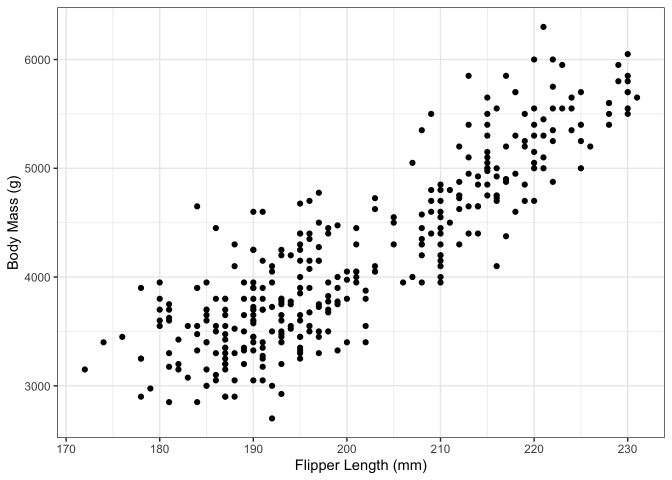
And then can add the regression line to it:
g_penguin_lm <- g_penguin +
    geom_abline(aes(slope=coef(penguin_lm)[2],
                  intercept=coef(penguin_lm)[1]))
g_penguin_lm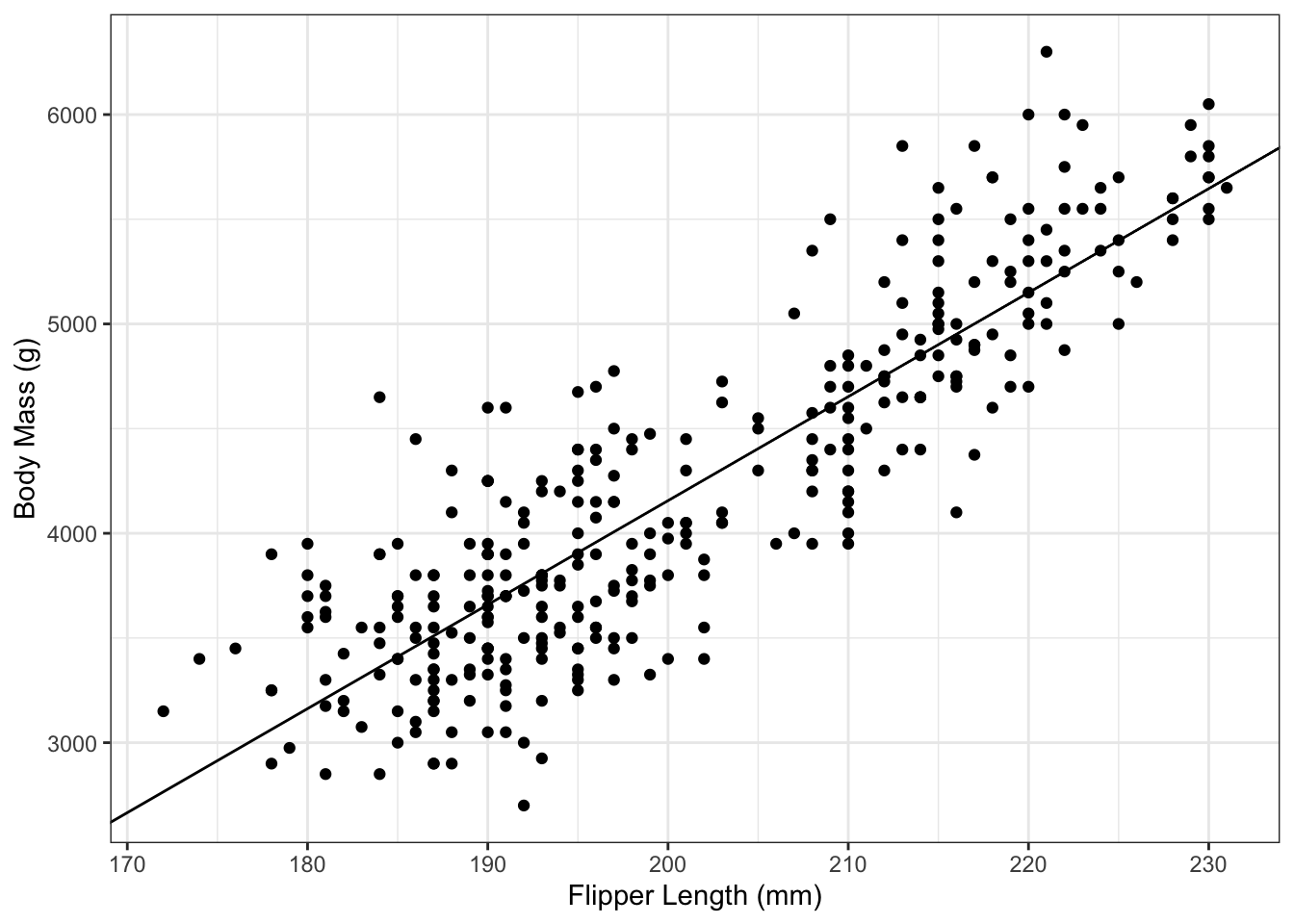
It’s important to remember to not type the numbers in directly. Not only does that lead to a loss of precision, it’s also greatly amplifies the chances of a typo. Instead, in the code above, we have used the coef() command to extract the slope and intercept estimates.
An alternative approach, which doesn’t actually require directly fitting the model, is to use the geom_smooth() command. To use this approach, provide that function
- an
xandyvariable inside theaes(), - the dataset via the
dataargument - set
method="lm"(Note the quotes), which tellsgeom_smooth()that you want the linear regression fit - optionally set
se=FALSE, which will hide the shaded uncertainty. We will later see how these are calculated in Section 5.
For example:
g_penguin_lm2 <-  g_penguin +
  geom_smooth(aes(x=flipper_length_mm,
                  y=body_mass_g),
              data=penguins,
              method="lm",
              se=FALSE)
g_penguin_lm2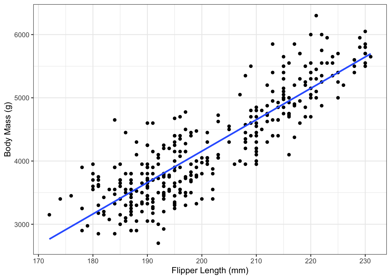
What happens if you forget method="lm"? In that case, the geom_smooth() function uses splines:
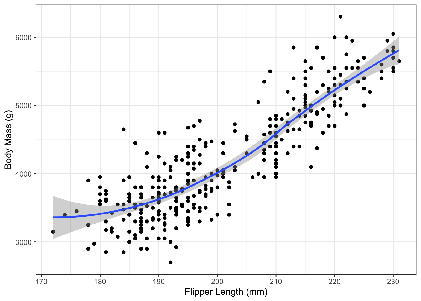
This an extremely useful method for visualizing the trend in a dataset. Just note that it is not the regression line.
Example 3.3 Consider the bike sharing data from Section 1.3.4 and Figure 1.9. After fitting an SLR model with temperature as the predictor variable and number of registered users as the outcome, we obtain the line:
\[ \hat y = 1370.9 + 112.4 x\] We can interpret these coefficients as:
- The estimated average number of registered users active in the bike sharing program on a day with high temperature 0 degrees Celsius is 1,371.
- A difference of one degree Celsius in daily high temperature is associated with an average of 112 more registered users actively renting a bike.
3.3.3 OLS estimation in R with binary x
If the predictor variable is a binary variable such as sex, then we need to create a corresponding 0-1 variable for fitting the model (recall Section 2.3.7). Conveniently, R will automatically create a 0-1 indicator from a binary categorical variable if that variable is included as a predictor in lm().
Example 3.4 (Continuation of Example 2.7.) Compute the OLS estimates of \(\beta_0\) and \(\beta_1\) for a linear regression model with penguin body mass as the outcome and penguin sex as the predictor variable.
We first restrict the dataset to penguins with known sex:
This ensures that our predictor can only take on two values (we will look at predictors with 3+ categories in Section 11).
We then call lm() using this dataset:
## (Intercept)     sexmale
##   3862.2727    683.4118
Note that R is providing an estimate labeled sexmale. The 0-1 indicator created by R automatically created the variable:
\[\begin{equation}
\texttt{sexmale} = \begin{cases} 0 & \text{ if } \texttt{sex} \text{ is } \texttt{"female"} \\ 1 & \text{ if } \texttt{sex} \text{ is } \texttt{"male"} \end{cases}.
\tag{3.6}
\end{equation}\]
In equation (3.6), female penguins were the reference category and received a value of 0. R chose female as the reference category (instead of male) simply because of alphabetical order.
We can write the following three interpretations of \(\hat\beta_0\), \(\hat\beta_0 + \hat\beta_1\), and \(\hat\beta_1\), respectively:
- The estimated average body mass for female penguins is 3,862 grams.
- The estimated average body mass for males penguins is 4,546 grams.
- The estimated difference in average body mass of penguins, comparing males to females, is 683 grams, with males having larger average mass.
3.4 Properties of Least Squares Estimators
3.4.1 Why OLS?
The reason OLS estimators \(\hat\beta_0\) and \(\hat\beta_1\) are so widely used is not only because they can be easily computed from the data, but also because they have good properties. Since \(\hat\beta_0\) and \(\hat\beta_1\) are random variables, they have a corresponding distribution.
We can compute the mean of \(\hat\beta_1\): \[\begin{align*} E\left[\hat\beta_1\right] & = E\left[\frac{S_{xy}}{S_x^2}\right]\\ &= \frac{1}{S_x^2}E\left[S_{xy}\right] \qquad \text{($S_x^2$ is not random)}\\ &= \frac{1}{S_x^2}E\left[\sum_{i=1}^n (x_i - \overline{x})y_i \right]\\ &= \frac{1}{S_x^2}\sum_{i=1}^n (x_i - \overline{x})E\left[y_i \right]\\ &= \frac{1}{S_x^2}\sum_{i=1}^n (x_i - \overline{x})(\beta_0 + \beta_1x_i)\\ &= \beta_0 \frac{\sum_{i=1}^n (x_i - \overline{x})}{S_x^2} + \beta_1\frac{\sum_{i=1}^n (x_i - \overline{x})x_i}{S_x^2}\\ &= \beta_0 \frac{n\overline{x}- n\overline{x}}{S_x^2} + \beta_1\frac{\sum_{i=1}^n x_i^2 - \frac{1}{n}\sum_{i=1}^n x_i \sum_{j=1}^n x_j}{S_x^2}\\ &= 0 + \beta_1 \frac{S_x^2}{S_x^2}\\ &= \beta_1 \end{align*}\] This means that \(\hat\beta_1\) is an unbiased estimator of \(\beta_1\). This is important since it means that, on average, using the OLS estimator \(\hat\beta_1\) will give us the “right” answer. Similarly, we can show that \(\hat\beta_0\) is unbiased: \[\begin{align*} \E\left[\hat\beta_0\right] &= \E\left[\frac{1}{n}\sum_{i=1}^ny_i - \hat\beta_1\frac{1}{n}\sum_{i=1}^nx_i\right]\\ &= \frac{1}{n}\sum_{i=1}^n\E[y_i] - \E[\hat\beta_1]\frac{1}{n}\sum_{i=1}^nx_i\\ &= \frac{1}{n}\sum_{i=1}^n(\beta_0 + \beta_1x_i) - \beta_1\frac{1}{n}\sum_{i=1}^nx_i\\ &= \frac{1}{n}\sum_{i=1}^n\beta_0 + \beta_1\left(\frac{1}{n} \sum_{i=1}^nx_i - \frac{1}{n}\sum_{i=1}x_i\right)\\ & = \beta_0 \end{align*}\]
However, it’s important to note that just because \(\E[\hat\beta_1] = \beta_1\) does not mean that \(\hat\beta_1 = \beta_1\). For a single data set, there is no guarantee that \(\hat\beta_1\) will be near \(\beta_1\). One way to measure how close \(\hat\beta_1\) is going to be to \(\beta_1\) is to compute its variance. The smaller the variance, the more likely that \(\hat\beta_1\) will be close to \(\beta_1\).
We can compute the variance of \(\hat\beta_1\) explicitly: \[\begin{align*} Var\left[\hat\beta_1\right] = \Var\left[\frac{S_{xy}}{S_x^2}\right] & = \frac{1}{(S_x^2)^2} Var\left[\sum_{i=1}^n (x_i - \overline{x}) y_i \right]\\ &= \frac{1}{(S_x^2)^2} \sum_{i=1}^n Var\left[(x_i - \overline{x}) y_i\right] \qquad \text{(Uncorrelated)}\\ &= \frac{1}{(S_x^2)^2} \sum_{i=1}^n(x_i - \overline{x})^2 Var\left[ y_i\right]\\ &= \frac{1}{(S_x^2)^2} \sum_{i=1}^n(x_i - \overline{x})^2 \sigma^2\\ &= \frac{1}{S_x^2} \sigma^2 \end{align*}\]
It can also be shown that \[ Var\left[\hat\beta_0\right] = \sigma^2\left(\frac{1}{n} + \frac{\overline{x}^2}{S_x^2}\right). \] Both \(\hat\beta_0\) and \(\hat\beta_1\) are linear estimators, because they are linear combinations of the data \(y_i\): \[\hat\beta_1 = \frac{S_{xy}}{S_x^2} = \sum_{i=1}^n \frac{ (x_i - \overline{x})}{S_x^2}y_i = \sum_{i=1}^n c_iy_i\]
The Gauss-Markov Theorem states that the OLS estimator has the smallest variance among linear unbiased estimators. It is the BLUE – Best Linear Unbiased Estimator.
In essence, the Gauss-Markov Theorem tells us that the OLS estimators are best we can do, at least as long as we only consider unbiased estimators. (We’ll see an alternative to this in Chapter 15).
3.5 Estimating \(\sigma^2\)
3.5.1 Not Regression: Estimating Sample Variance
Before discussing how to estimate \(\sigma^2\) in SLR, it’s helpful to first recall how we estimate the variance from a sample of a single random variable.
Suppose \(y_1, y_2, \dots, y_n\) are iid samples from a distribution with mean \(\mu\) and variance \(\sigma^2\). The estimated mean is:
\[\overline{y} = \frac{1}{n}\sum_{i=1}^n y_i\]
and the estimated variance is:
\[s^2 = \frac{1}{n - 1}\sum_{i=1}^n (y_i - \overline{y})^2\]
In \(s^2\), why do we divide by \(n-1\)? To understand this, first consider what would happen if we divided by \(n\) instead: \[\begin{align*} E\left[\frac{1}{n}\sum_{i=1}^n(Y_i - \overline{Y})^2\right] &= E \left[ \frac{1}{n} \sum_{i=1}^n (Y_i - \mu + \mu - \overline{Y})^2 \right]\\ &= E \left[ \frac{1}{n} \sum_{i=1}^n \left((Y_i - \mu)^2 + 2(Y_i - \mu)(\mu - \overline{Y}) + (\mu - \overline{Y})^2\right) \right] \\ &= \frac{1}{n} \sum_{i=1}^n E\left[(Y_i - \mu)^2 \right] - \frac{2}{n}E\left[\sum_{i=1}^n (Y_i - \mu)(\overline{Y} - \mu) \right] + \frac{1}{n}E\left[(\overline{Y} - \mu)^2 \right]\\ &= \frac{1}{n} \sum_{i=1}^n \sigma^2 - \frac{2}{n}E\left[\sum_{i=1}^n (Y_i - \mu) \frac{1}{n}\sum_{j=1}^n (Y_j - \mu) \right] + \frac{1}{n}\sum_{i=1}^n \frac{\sigma^2}{n}\\ &= \sigma^2 - \frac{2}{n^2}\sum_{i=1}^n\sum_{j=1}^n E\left[(Y_i - \mu)(Y_j - \mu)\right] + \sigma^2/n\\ &= \sigma^2 - \frac{2}{n^2} \sum_{i=1}^nE\left[(Y_i - \mu)^2 \right] - \frac{2}{n^2} \sum_{i=1}^n\sum_{j=1, j\ne i}^n E \left[ (Y_i - \mu)(Y_j - \mu) \right] + \sigma^2/n\\ &= \sigma^2 - \frac{2}{n}\sigma^2 + \frac{1}{n}\sigma^2\\ &= \sigma^2\left(1 - \frac{1}{n}\right)\\ &= \frac{n-1}{n} \sigma^2 \end{align*}\] This estimator is biased by a factor of \(\frac{n-1}{n}\). If we instead divide by \(n-1\), then we obtain an unbiased estimator: \[\E\left[\frac{1}{n-1}\sum_{i=1}^n(Y_i - \overline{Y})^2 \right] = \frac{n}{n-1} \E\left[\frac{1}{n}\sum_{i=1}^n(Y_i - \overline{Y})^2 \right] = \frac{n}{n-1}\frac{n-1}{n}\sigma^2=\sigma^2\]
That explains the mathematical reason for dividing by \(n-1\). But what is the conceptual rationale? The answer is degrees of freedom. The full sample contains \(n\) values. Computing the estimator \(s^2\) requires first computing the sample mean \(\overline{y}\). This “uses up” one degree of freedom, meaning that only \(n-1\) degrees of freedom are left when computing \(s^2\).
This is perhaps easier to see with an example. Suppose \(n=5\). If \(\overline{y} = 7\) and \(y_1=3, y_2=1, y_3=8, y_4=10\). What is \(y_5\)? It must be that \(y_5=10\). Knowing \(\overline{y}\) determines \(\sum_{i=1}^n y_i\). In this way, computing \(\overline{y}\) puts a constraint on what the possible values of the data can be.
3.5.2 Estimating \(\sigma^2\) in SLR
Now, back to SLR. We want to estimate \(\sigma^2\). Because \(\Var(\epsilon_i) = \sigma^2\) and \(\E[\epsilon_i] = 0\), it follows that \[\E[\epsilon_i^2] = \Var(\epsilon_i) + \E[\epsilon_i]^2 = \sigma^2 + 0 = \sigma^2.\] Thus, an estimate of \(\E[\epsilon_i^2]\) is an estimate of \(\sigma^2\). A natural estimator of \(\E[\epsilon_i^2]\) is \[\hat\sigma^2 = \frac{1}{n-2}\sum_{i=1}^n e_i^2\] Why divide by \(n-2\) here? Since \(e_i = y_i - (\hat\beta_0 + \hat\beta_1x_i)\), there are 2 degrees of freedom used up in computing the residuals \(e_i\).
\(\sum_{i=1}^n\limits e_i^2 = SS_{res}\) is called the “sum of squared residuals” or “residual sum of squares”
\(\hat\sigma^2 = MS_{res}\) is called “mean squared residuals”
3.5.3 Estimating \(\sigma^2\) in R
When summary() is called on an lm object, the sigma slot provides \(\hat\sigma\) for you:
## [1] 394.2782## [1] 155455.3The value of \(\hat\sigma\) is also printed in the summary output:
##
## Call:
## lm(formula = body_mass_g ~ flipper_length_mm, data = penguins)
##
## Residuals:
##      Min       1Q   Median       3Q      Max
## -1058.80  -259.27   -26.88   247.33  1288.69
##
## Coefficients:
##                    Estimate Std. Error t value Pr(>|t|)
## (Intercept)       -5780.831    305.815  -18.90   <2e-16 ***
## flipper_length_mm    49.686      1.518   32.72   <2e-16 ***
## ---
## Signif. codes:  0 '***' 0.001 '**' 0.01 '*' 0.05 '.' 0.1 ' ' 1
##
## Residual standard error: 394.3 on 340 degrees of freedom
##   (2 observations deleted due to missingness)
## Multiple R-squared:  0.759,  Adjusted R-squared:  0.7583
## F-statistic:  1071 on 1 and 340 DF,  p-value: < 2.2e-16
It’s also possible to compute this value “by hand” in R:
## [1] 155455.3## [1] 394.27823.6 Exercises
Exercise 3.1 Fit an SLR model to the bill size data among Gentoo penguins, using bill length as the predictor and bill depth as the outcome. Find \(\hat\beta_0\) and \(\hat\beta_1\) using the formulas and then compare to the value calculated by lm().
Exercise 3.2 Using the mpg data (see Section 1.3.5), use lm() to find the estimates of \(\hat\beta_0\) and \(\hat\beta_1\) for a SLR model with city highway miles per gallon as the outcome variable and engine displacement as the predictor variable. Provide a one-sentence interpreation of each estimate.
Exercise 3.3 Compute \(\hat\sigma^2\) for the model in Exercise 3.2 using the formulas. Compare to the value calculated from the lm object.
Exercise 3.4 Consider the housing price data introduced in Section 1.3.3, with housing price as the outcome and median income as the predictor variable. Find the OLS estimates for a simple linear regression analysis of this data and provide a 1-sentence interpretation for each.
In most cases, we suppress the dependence on \(\hat\beta_0\) and \(\hat\beta_1\) and just write \(SS_{Res}\). But the dependence is included here to make the optimization explicit.↩︎